


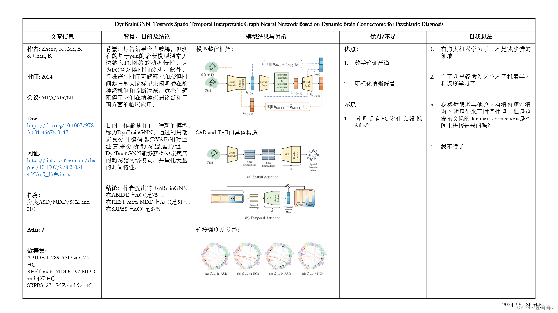
 论文提出了一种名为DynBrainGNN的模型,利用动态脑连接组和变分自编码器,解决了精神疾病诊断中动态模型缺乏解释性的挑战。模型结合了空间注意力和时间注意力机制,提供了疾病特异性大脑动态网络连接和时间属性的解释。实验在多个数据集上展示了其在分类性能上的优势。
论文全名:DynBrainGNN: Towards Spatio-Temporal Interpretable Graph Neural Network Based on Dynamic Brain Connectome for Psychiatric Diagnosis
英文是纯手打的!论文原文的summarizing and paraphrasing。可能会出现难以避免的拼写错误和语法错误,若有发现欢迎评论指正!文章偏向于笔记,谨慎食用
目录
2.3.2. Overall Framework of DynBrainGNN
2.3.3. Construction of Dynamic Functional Graph
2.3.5. Spatio-Temporal Attention-Based READOUT Module
2.3.6. Dynamic Variational Autoencoders (DVAE)
2.4.4. Evaluation on Classification Performance
2.5.1. Disease-Specific Brain Dynamic Network Connections
1. 省流版
1.1. 心得
(1)完了写完了才发现没有心得,那我咋总结啊?
1.2. 论文总结图
2. 论文逐段精读
2.1. Abstract
①Again, FC can not present the dynamic character of fMRI
elucidate v.阐明;说明;解释
2.2. Introduction
①⭐They challenge that the exist dynamic models lack interpretability in dwell time, fractional windows and number of transitions(意思你能解决?)
②They propose a Dynamic Brain Graph Neural Networks (DynBrainGNN), which based on dynamic brain connectom via dynamic variational autoencoders (DVAE) and spatio-temporal attention
③It is the first time that someone put forward such a "build in" dynamic FC?(啥玩意?真真第一次?)
2.3. Proposed Model
2.3.1. Problem Definition
①Graph set: , where
is the time series with
length of the
-th subject and
is the number of subjects
②Through graphs, they extract and learn features
③The real label set:
2.3.2. Overall Framework of DynBrainGNN
①The schematic of DynBrainGNN:
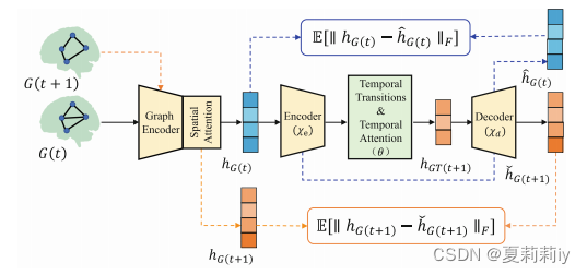
which covers graph encoder, spatial attention module, temporal attention module and DVAE four modules;
where decoder recovers and
;
然后,作者只是说橙色蓝色那俩框框是“为了保证解码器的可靠”,然后也没多说了
2.3.3. Construction of Dynamic Functional Graph
①Length of time series:
②Length of slicing window:
③Stride:
④By dynamic cutting, they obtain windowed dFC matrices(为啥?如果T=10,L=8,S=1,W不就等于2了吗,但是看上去是不是有1-8,2-9,3-10三个啊,不会要加一吗?)
⑤Each dFC calculated by Pearson correlation
⑥⭐They get the graph where
is a adjacency matrix that all 1 transformed by the top 20% absolute correlation and
denotes the node features which constructed by the row or column of FC matrix
2.3.4. Graph Encoder
①Graph encoder: GCN
②Propagation rule of GCN:
where ,
denotes learnable parameters and
denotes Sigmoid
2.3.5. Spatio-Temporal Attention-Based READOUT Module
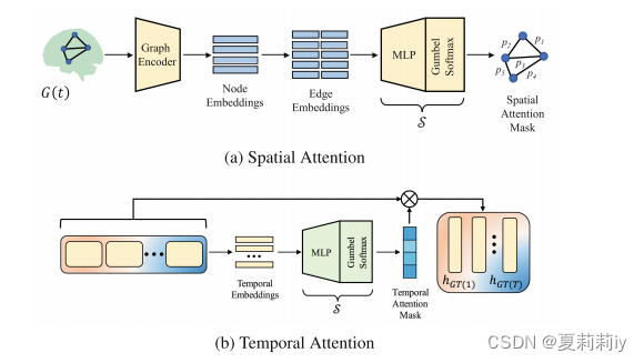
①They designed two attention based READOUT methods, Spatial Attention READOUT (SAR) and Temporal Attention READOUT (TAR)
②Based on prior , they define
③In SAR, , where
denotes concatenation
④In TAR, is constructed by the concatenation of several graph presentations at different times
⑤The specific operation of :
after Sigmoid, . "Then, attention masks are sampled from Bernoulli distributions, and the gumbelsoftmax reparameterization trick is applied to update
"
⑥In SAR,
⑦In TAR, where
denotes Kronecker product
⑧Schematic of SAR and TAR:
2.3.6. Dynamic Variational Autoencoders (DVAE)
①Temporal transition:
②The function of DVAE:
where ,
represents the encoder model(什么东西啊?就是GCN吗?),
indicates the Frobenius norm,
denotes the prior distribution with isotropic Gaussian (assumed),
and
are both scaling coefficients of the regularization term
③One more regularization term for compacting:
where denotes the matrix-based Renyi’s
-order mutual information and
denotes the scaling coefficient
④Accordingly, combining them all to get a final loss function, where
is cross entropy loss
2.4. Experiments
2.4.1. Dataset
①ABIDE I: 289 ASD and 23 HC for no reason
②REST-meta-MDD: 397 MDD and 427 HC
③SRPBS: " This is a multi-disorder MRI dataset"(吓我一跳,总感觉是同时身患玉玉症多动症焦虑症自闭症老年痴呆的被试呢), selecting 234 SCZ and 92 HC
2.4.2. Baselines
①Settings:
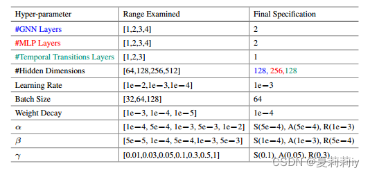
2.4.3. Experimental Settings
①Cross validation: 5 fold
②Decision of hyper-parameter: grid search
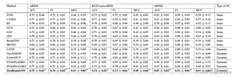
2.4.4. Evaluation on Classification Performance
①Comparison table:
2.5. Interpretation Analysis
2.5.1. Disease-Specific Brain Dynamic Network Connections
①The interpretations of dynamically dominant and fluctuant connections(?)are brought by and
②They define dominant subgraph and fluctuant subgraph
:
where and
is the mean value of
③The top 50 influential edges:
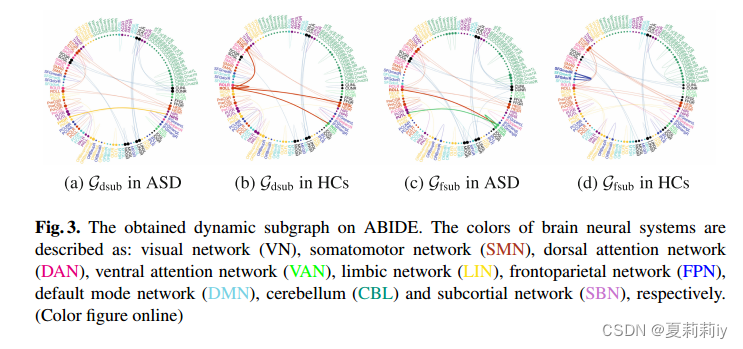
sensorimotor adj. 感觉运动的(等于 sensomotor)
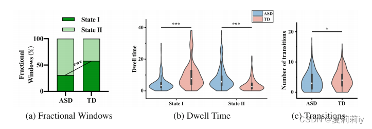
2.5.2. Temporal Properties
①“我们提供的时间属性的解释,以了解大脑的灵活性和适应性在精神疾病。具体而言,我们首先应用k-means聚类算法对有窗时空参与的图表示hGT进行聚类,以评估动态大脑模式(状态)。使用基于轮廓分数的聚类有效性分析来确定最佳聚类数量。然后,我们量化这些状态的时间属性的组差异,包括停留时间(即属于一个状态的连续窗口的持续时间),分数窗口(即属于一个状态的总窗口的比例)和转换数量(即状态之间的转换数量)。使用带有错误发现率(FDR)校正的双样本t检验(图4)。我们的分析显示,ASD患者在II状态下有更高的分数窗口和平均停留时间,这与最近的一项神经影像学研究一致”(我失去了paraphrase能力)
②Temporal properties:
2.5.3. Conclusion
They want to further try their model in other datasets
3. 知识补充
3.1. Dwell time
搜了一圈没搜到关于医学设备的,提供以下猜测
(1)最可能的,length of time series signals
(2)两个相邻点之间的时间?比如task fMRI两次task之间的时间间隔
(3)嘻嘻,事实证明上面俩都是错的,在2.5.2.作者说它是"the duration of consecutive windows belonging to one state"
4. Reference List
Zheng, K., Ma, B. & Chen, B. (2024) 'DynBrainGNN: Towards Spatio-Temporal Interpretable Graph Neural Network Based on Dynamic Brain Connectome for Psychiatric Diagnosis', Machine Learning in Medical Imaging, 14349.doi: DynBrainGNN: Towards Spatio-Temporal Interpretable Graph Neural Network Based on Dynamic Brain Connectome for Psychiatric Diagnosis | SpringerLink


 5903
5903

 被折叠的 条评论
为什么被折叠?
被折叠的 条评论
为什么被折叠?
 到【灌水乐园】发言


