


目录
本文是对SPLUT技术的代码解读,原文解读请看SPLUT。
原文概要
SPLUT通过增大网络感受野,来提升超分效果,实现SRLUT的改进,主要两个创新点:
- 提出了一个无需旋转集成、多LUT串联和并联的方法来提升感受野。
- 提出了一个并行网络做补偿,来改善LUT的量化误差问题。
其网络结构图如下:
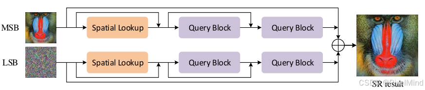
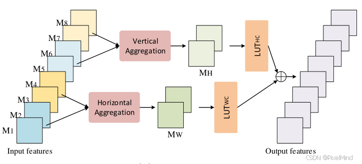
Query Blocks:
代码结构如下:
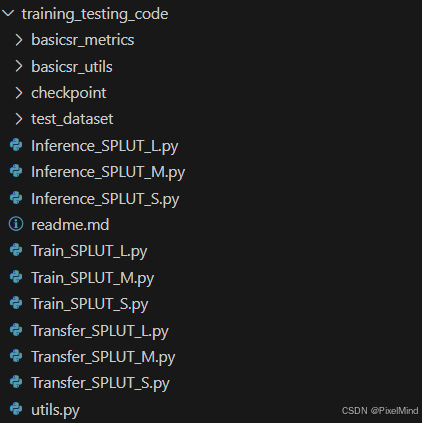
我们这里以后缀为M的SPLUT为例进行讲解。
1. 训练
代码位于Train_SPLUT_M.py文件中,某一个分支结构实现如下,MSB和LSB都会经过下面的结构,处理后相加就得到最终结果,跟前面讲到的结构是对应的:
class SRNet(torch.nn.Module):
    def __init__(self, upscale=4):
        super(SRNet, self).__init__()

        self.upscale = upscale
        self.lvls = 16
        self.quant= BASEQ(self.lvls ,8.0)
        self.out_channal= OUT_NUM

        #cwh
        self.lut122=nn.Sequential(
            nn.Conv2d(1, 64, [2,2], stride=1, padding=0, dilation=1),
            nn.GELU(),
            nn.Conv2d(64, 64, 1, stride=1, padding=0, dilation=1),
            nn.GELU(),
            nn.Conv2d(64, 8, 1, stride=1, padding=0, dilation=1)
        )

        self.lut221=nn.Sequential(
            nn.Conv2d(2,  64, [2,1], stride=1, padding=0, dilation=1),
            nn.GELU(),
            nn.Conv2d(64, 64, 1, stride=1, padding=0, dilation=1),
            nn.GELU(),
            nn.Conv2d(64, 64, 1, stride=1, padding=0, dilation=1),
            nn.GELU(),
            nn.Conv2d(64, 8, 1, stride=1, padding=0, dilation=1)
        )

        self.lut212=nn.Sequential(
            nn.Conv2d(2,  64, [1,2], stride=1, padding=0, dilation=1),
            nn.GELU(),
            nn.Conv2d(64, 64, 1, stride=1, padding=0, dilation=1),
            nn.GELU(),
            nn.Conv2d(64, 64, 1, stride=1, padding=0, dilation=1),
            nn.GELU(),
            nn.Conv2d(64, 8, 1, stride=1, padding=0, dilation=1)
        )

        self.lut221_c12=nn.Sequential(
            nn.Conv2d(2,  64, [2,1], stride=1, padding=0, dilation=1),
            nn.GELU(),
            nn.Conv2d(64, 64, 1, stride=1, padding=0, dilation=1),
            nn.GELU(),
            nn.Conv2d(64, 64, 1, stride=1, padding=0, dilation=1),
            nn.GELU(),
            nn.Conv2d(64, 16, 1, stride=1, padding=0, dilation=1)
        )

        self.lut212_c34=nn.Sequential(
            nn.Conv2d(2,  64, [1,2], stride=1, padding=0, dilation=1),
            nn.GELU(),
            nn.Conv2d(64, 64, 1, stride=1, padding=0, dilation=1),
            nn.GELU(),
            nn.Conv2d(64, 64, 1, stride=1, padding=0, dilation=1),
            nn.GELU(),
            nn.Conv2d(64, 16, 1, stride=1, padding=0, dilation=1)
        )

        self.pixel_shuffle = nn.PixelShuffle(upscale)

        # Init weights
        for m in self.modules():
            classname = m.__class__.__name__
            if classname.lower().find('conv') != -1:
                nn.init.kaiming_normal(m.weight)
                nn.init.constant(m.bias, 0)
            elif classname.find('bn') != -1:
                m.weight.data.normal_(1.0, 0.02)
                m.bias.data.fill_(0)

    def forward(self, x_in):
        B, C, H, W = x_in.size()
        x_in = x_in.reshape(B*C, 1, H, W)
        x = self.lut122(x_in)+x_in[:,:,:H-1,:W-1]
        x_temp=x_in
        x221 = self.lut221(self.quant(F.pad(x[:,0:2,:,:],(0,0,0,1), mode='reflect')+F.pad(x[:,2:4,:,:],(0,0,1,0), mode='reflect')))
        x212 = self.lut212(self.quant(F.pad(x[:,4:6,:,:],(0,1,0,0), mode='reflect')+F.pad(x[:,6: ,:,:],(1,0,0,0), mode='reflect')))
        x=(x221+x212)/2.0+x

        x2 = self.lut221_c12(self.quant(F.pad(x[:,0:2,:,:],(0,0,0,1), mode='reflect')+F.pad(x[:,2:4,:,:],(0,0,1,0), mode='reflect')))
        x3 = self.lut212_c34(self.quant(F.pad(x[:,4:6,:,:],(0,1,0,0), mode='reflect')+F.pad(x[:,6: ,:,:],(1,0,0,0), mode='reflect')))
        x=(x2+x3)/2.0+x_temp[:,:,:H-1,:W-1]
        x = self.pixel_shuffle(x)
        x = x.reshape(B, C, self.upscale*(H-1), self.upscale*(W-1))
return x可以看到self.lut122代表了空间的lut,即Spatial Lookup。
接下来计算x221,先忽略quant算子,可以看到F.pad(x[:,0:2,:,:],(0,0,0,1), mode='reflect')+F.pad(x[:,2:4,:,:],(0,0,1,0), mode='reflect'),这个过程代表了Query Blocks里的horizontal aggregate模块。再进行LUT221,即LUT WC的操作,这样子完成Query Blocks的一个支路。x212即是对应的vertical部分,这两部分加起来之后除以2即可。
接下来是重复的计算x2和x3,最后经过一个pixel_shuffle完成超分即可。
然后是量化节点的实现,代码如下:
class _baseq(torch.autograd.Function):
    @staticmethod
    def forward(ctx, x, steps):
        y_step_ind=torch.floor(x / steps)
        y = y_step_ind * steps
        return y

    @staticmethod
    def backward(ctx, grad_output):
        return grad_output, None

class BASEQ(nn.Module):
    def __init__(self, lvls,activation_range):
        super(BASEQ, self).__init__()
        self.lvls = lvls
        self.activation_range = activation_range
        self.steps = 2 * activation_range / self.lvls

    def forward(self, x):
        x=(((-x - self.activation_range).abs() - (x - self.activation_range).abs()))/2.0
        x[x > self.activation_range-0.1*self.steps] =self.activation_range-0.1*self.steps
return _baseq.apply(x, self.steps)量化节点是这个BASEQ类,作者给的lvls和activation_range的默认值分别是16和8,因此steps就是1,前向第一步是等价一个torch.clip操作,大于activation range是activation range,小于-activation range是-activation range,在-activation range和activation range之间是x(这里可以将不同情况下的输入带入代码中计算,可以得到这个结论),第二步博主这里认为是由于带符号数正数和负数是不对称的,例如一个4bit的输入,它的值域范围是[-8, 7],因此这里对正数做了进一步的clip,来减小这个误差。最后应用_baseq的量化算子,因为steps是1,这里Funcition的forward完成的是一个向下取整的floor操作,backward完成的就是STE,直接将梯度传递下去,保证整个网络的可导性。
2. 转表
在Transfer_SPLUT_M.py中,这里跟SRLUT基本一致,根据LUT类型,先构造4bit的输入,如下:
L = 2 ** img_bits
 base_step_ind=torch.arange(0, L, 1)
 base=base_step_ind/16.0
 index_4D=torch.meshgrid(base,base,base,base)
 onebyfourth=torch.cat([index_4D[0].flatten().unsqueeze(1),index_4D[1].flatten().unsqueeze(1),index_4D[2].flatten().unsqueeze(1),index_4D[3].flatten().unsqueeze(1)],1)

 base_B=base_step_ind/16.0
 index_4D_B=torch.meshgrid(base_B,base_B,base_B,base_B)
 onebyfourth_B=torch.cat([index_4D_B[0].flatten().unsqueeze(1),index_4D_B[1].flatten().unsqueeze(1),index_4D_B[2].flatten().unsqueeze(1),index_4D_B[3].flatten().unsqueeze(1)],1)

if LUT_NUM==1:
    input_tensor   = onebyfourth.unsqueeze(1).unsqueeze(1).reshape(-1,1,2,2)
    input_tensor_B = onebyfourth_B.unsqueeze(1).unsqueeze(1).reshape(-1,1,2,2)
elif KERNAL==221:
    input_tensor = onebyfourth.unsqueeze(1).unsqueeze(1).reshape(-1,2,2,1)
    input_tensor_B = onebyfourth.unsqueeze(1).unsqueeze(1).reshape(-1,2,2,1)
elif KERNAL==212:
    input_tensor = onebyfourth.unsqueeze(1).unsqueeze(1).reshape(-1,2,1,2)
    input_tensor_B = onebyfourth.unsqueeze(1).unsqueeze(1).reshape(-1,2,1,2)
再送入之前训练好的层中输出结果并将其保存即可。
3. 测试
在Inference_SPLUT_M.py中,这里只是将网络的部分用LUT表去实现了,而且前面也讲到了,SPLUT是4bit的,不用量化,所以它的测试中不存在插值,所以与网络推理的代码就非常相像了。如下:
 img_in = np.pad(img_lr, ((0,1), (0,1), (0,0)), mode='reflect').transpose((2,0,1))
    img_in_A255 = img_in// L
    img_in_B255 = img_in % L
    img_in_A = img_in_A255/L
    img_in_B = img_in_B255/L

    # A
    x_layer1=LUT1_122(LUTA1_122,img_in_A255)+img_in_A[:,0:h,0:w].reshape((3,1,h,w))
    x2_in1=np.pad(x_layer1[:,0:2,:,:],((0,0),(0,0),(0,1),(0,0)), mode='reflect')+np.pad(x_layer1[:,2:4,:,:],((0,0),(0,0),(1,0),(0,0)), mode='reflect')
    x2_in2=np.pad(x_layer1[:,4:6,:,:],((0,0),(0,0),(0,0),(0,1)), mode='reflect')+np.pad(x_layer1[:,6: ,:,:],((0,0),(0,0),(0,0),(1,0)), mode='reflect')
    x_layer2=(LUT23(LUTA2_221, x2_in1,8.0 ,'k221',2)+LUT23(LUTA2_212, x2_in2,8.0 ,'k212',2))/2.0+x_layer1
    x3_in1=np.pad(x_layer2[:,0:2,:,:],((0,0),(0,0),(0,1),(0,0)), mode='reflect')+np.pad(x_layer2[:,2:4,:,:],((0,0),(0,0),(1,0),(0,0)), mode='reflect')
    x3_in2=np.pad(x_layer2[:,4:6,:,:],((0,0),(0,0),(0,0),(0,1)), mode='reflect')+np.pad(x_layer2[:,6: ,:,:],((0,0),(0,0),(0,0),(1,0)), mode='reflect')
    img_out=(LUT23(LUTA3_221, x3_in1,8.0 ,'k221',3)+LUT23(LUTA3_212, x3_in2,8.0 ,'k212',3))/2.0+img_in_A[:,0:h,0:w].reshape((3,1,h,w))
    img_out=img_out.reshape((3,UPSCALE,UPSCALE,h,w))
    img_out=np.transpose(img_out,(0,3,1,4,2)).reshape((3,UPSCALE*h,UPSCALE*w))
    img_out_A = img_out.transpose((1,2,0))
    # B
    x_layer1=LUT1_122(LUTB1_122,img_in_B255)+img_in_B[:,0:h,0:w].reshape((3,1,h,w))
    x2_in1=np.pad(x_layer1[:,0:2,:,:],((0,0),(0,0),(0,1),(0,0)), mode='reflect')+np.pad(x_layer1[:,2:4,:,:],((0,0),(0,0),(1,0),(0,0)), mode='reflect')
    x2_in2=np.pad(x_layer1[:,4:6,:,:],((0,0),(0,0),(0,0),(0,1)), mode='reflect')+np.pad(x_layer1[:,6: ,:,:],((0,0),(0,0),(0,0),(1,0)), mode='reflect')
    x_layer2=(LUT23(LUTB2_221, x2_in1,8.0 ,'k221',2)+LUT23(LUTB2_212, x2_in2,8.0 ,'k212',2))/2.0+x_layer1
    x3_in1=np.pad(x_layer2[:,0:2,:,:],((0,0),(0,0),(0,1),(0,0)), mode='reflect')+np.pad(x_layer2[:,2:4,:,:],((0,0),(0,0),(1,0),(0,0)), mode='reflect')
    x3_in2=np.pad(x_layer2[:,4:6,:,:],((0,0),(0,0),(0,0),(0,1)), mode='reflect')+np.pad(x_layer2[:,6: ,:,:],((0,0),(0,0),(0,0),(1,0)), mode='reflect')
    img_out=(LUT23(LUTB3_221, x3_in1,8.0 ,'k221',3)+LUT23(LUTB3_212, x3_in2,8.0 ,'k212',3))/2.0+img_in_B[:,0:h,0:w].reshape((3,1,h,w))
    img_out=img_out.reshape((3,UPSCALE,UPSCALE,h,w))
    img_out=np.transpose(img_out,(0,3,1,4,2)).reshape((3,UPSCALE*h,UPSCALE*w))
    img_out_B = img_out.transpose((1,2,0))

    img_out=img_out_A+img_out_B
    img_out = np.round(np.clip(img_out, 0, 1) * 255).astype(np.uint8)
可见,开始先获取MSB和LSB,然后送入LUT表中推理,过程跟我们前面的网络的推理过程是非常相像的,数据只不过是numpy.array和torch.Tensor的区别。


 2187
2187

 被折叠的 条评论
为什么被折叠?
被折叠的 条评论
为什么被折叠?
 到【灌水乐园】发言


