【lssvm预测】基于粒子群优化lssvm实现预测matlab源码

最新推荐文章于 2025-12-02 19:45:00 发布

原创最新推荐文章于 2025-12-02 19:45:00 发布 · 54 阅读

0 ·

CC 4.0 BY-SA版权

文章标签：

#matlab #算法 #开发语言

一、粒子群算法的基本思想

设想这样一个场景：一群鸟在随机搜索食物。已知在这块区域里只有一块食物；所有的鸟都不知道食物在哪里；但它们能感受到当前的位置离食物还有多远。那么找到食物的最优策略是什么呢？

1. 搜寻目前离食物最近的鸟的周围区域

2. 根据自己飞行的经验判断食物的所在。

PSO正是从这种模型中得到了启发，PSO的基础是信息的社会共享

算法介绍

每个寻优的问题解都被想像成一只鸟，称为“粒子”。所有粒子都在一个D维空间进行搜索。

所有的粒子都由一个fitness function 确定适应值以判断目前的位置好坏。

每一个粒子必须赋予记忆功能，能记住所搜寻到的最佳位置。

每一个粒子还有一个速度以决定飞行的距离和方向。这个速度根据它本身的飞行经验以及同伴的飞行经验进行动态调整。

【lssvm预测】基于粒子群优化lssvm实现预测matlab源码_粒子群算法

【lssvm预测】基于粒子群优化lssvm实现预测matlab源码_粒子群算法_02

　　粒子速度更新公式包含三部分：第一部分为“惯性部分”，即对粒子先前速度的记忆；第二部分为“自我认知”部分，可理解为粒子i当前位置与自己最好位置之间的距离；第三部分为“社会经验”部分，表示粒子间的信息共享与合作，可理解为粒子i当前位置与群体最好位置之间的距离。

粒子群算法流程

第1步在初始化范围内，对粒子群进行随机初始化，包括随机位置和速度

第2步计算每个粒子的适应值

第3步更新粒子个体的历史最优位置

第4步更新粒子群体的历史最优位置

第5步更新粒子的速度和位置

第6步若未达到终止条件，则转第2步

　　粒子群算法流程图如下：

【lssvm预测】基于粒子群优化lssvm实现预测matlab源码_粒子群算法_03

二、lssvm

1、最小二乘支持向量机LSSVM基本原理

最小二乘支持向量机是支持向量机的一种改进，它是将传统支持向量机中的不等式约束改为等式约束, 且将误差平方和(SumSquaresError)损失函数作为训练集的经验损失,这样就把解二次规划问题转化为求解线性方程组问题, 提高求解问题的速度和收敛精度。

常用的核函数种类：

【lssvm预测】基于粒子群优化lssvm实现预测matlab源码_粒子群算法_04

三、代码

%=====================================================================
%初始化
clc
close all
clear
format long


tic
%==============================================================
%%导入数据
data=xlsread('1.xlsx');
[row,col]=size(data);
x=data(:,1:col-1);
y=data(:,col);
set=1; %设置测量样本数
row1=row-set;%
train_x=x(1:row1,:);
train_y=y(1:row1,:);
test_x=x(row1+1:row,:);%预测输入
test_y=y(row1+1:row,:);%预测输出
train_x=train_x';
train_y=train_y';
test_x=test_x';
test_y=test_y';

%%数据归一化
[train_x,minx,maxx, train_yy,miny,maxy] =premnmx(train_x,train_y);
test_x=tramnmx(test_x,minx,maxx);


train_x=train_x';
train_yy=train_yy';
train_y=train_y';
test_x=test_x';
test_y=test_y';



%% 参数初始化

%粒子群算法中的两个参数
c1 = 1.5;%; % c1 belongs to [0,2] c1:初始为1.5,pso参数局部搜索能力，表征个体极值对当前解得影响
c2 = 1.7;%; % c2 belongs to [0,2] c2:初始为1.7,pso参数全局搜索能力，表征全局极值对当前解得影响

maxgen=100; % 进化次数 300
sizepop=20; % 种群规模30

popcmax=10^(3);% popcmax:初始为1000,SVM 参数c的变化的最大值.
popcmin=10^(-1);% popcmin:初始为0.1,SVM 参数c的变化的最小值.
popgmax=10^(2);% popgmax:初始为100,SVM 参数g的变化的最大值
popgmin=10^(-2);% popgmin:初始为0.01,SVM 参数g的变化的最小值.
k = 0.5; % k belongs to [0.1,1.0];
Vcmax = k*popcmax;%参数 c 迭代速度最大值
Vcmin = -Vcmax ;
Vgmax = k*popgmax;%参数 g 迭代速度最大值
Vgmin = -Vgmax ; 

eps = 10^(-6);

wVmax=1;
wVmin=0.01;

%%定义lssvm相关参数
type='f';
kernel = 'RBF_kernel';
proprecess='proprecess';

%% 产生初始粒子和速度
for i=1:sizepop

% 随机产生种群
pop(i,1) = (popcmax-popcmin)*rand(1,1)+popcmin ; % 初始种群
pop(i,2) = (popgmax-popgmin)*rand(1,1)+popgmin;
V(i,1)=Vcmax*rands(1,1); % 初始化速度
V(i,2)=Vgmax*rands(1,1);

% 计算初始适应度
gam=pop(i,1);
sig2=pop(i,2);
model=initlssvm(train_x,train_yy,type,gam,sig2,kernel,proprecess);
model=trainlssvm(model);
%求出训练集和测试集的预测值
[train_predict_y,zt,model]=simlssvm(model,train_x);
[test_predict_y,zt,model]=simlssvm(model,test_x);
%预测数据反归一化
train_predict=postmnmx(train_predict_y ,miny,maxy);%预测输出
test_predict=postmnmx(test_predict_y ,miny,maxy); %测试集预测值
%计算均方差

trainmse=sum((train_predict-train_y).^2)/length(train_y);
testmse=sum((test_predict-test_y).^2)/length(test_y); 
fitness(i)=trainmse; %以测试集的预测值计算的均方差为适应度值
end

% 找极值和极值点
[global_fitness bestindex]=min(fitness); % 全局极值
local_fitness=fitness; % 个体极值初始化 

global_x=pop(bestindex,:) % 全局极值点
local_x=pop; % 个体极值点初始化

% 每一代种群的平均适应度
avgfitness_gen = zeros(1,maxgen);



%% 迭代寻优
for i=1:maxgen
i

for j=1:sizepop

%速度更新
%wV =wVmax-(wVmax-wVmin)/maxgen/maxgen*i*i   二次递减策略
%wV =wVmax-(wVmax-wVmin)/maxgen*i   %线性递减策略
wV = 1; % wV best belongs to [0.8,1.2]为速率更新公式中速度前面的弹性系数，上一个速度/位置对当前速度/位置的影响
V(j,:) = wV*V(j,:) + c1*rand*(local_x(j,:) - pop(j,:)) + c2*rand*(global_x - pop(j,:));
if V(j,1) > Vcmax %以下几个不等式是为了限定速度在最大最小之间
V(j,1) = Vcmax;
end
if V(j,1) < Vcmin
V(j,1) = Vcmin;
end
if V(j,2) > Vgmax
V(j,2) = Vgmax;
end
if V(j,2) < Vgmin
V(j,2) = Vgmin; %以上几个不等式是为了限定速度在最大最小之间
end

%种群更新
wP = 1; % wP:初始为1,种群更新公式中速度前面的弹性系数
pop(j,:)=pop(j,:)+wP*V(j,:);
if pop(j,1) > popcmax %以下几个不等式是为了限定 c 在最大最小之间
pop(j,1) = popcmax;
end
if pop(j,1) < popcmin
pop(j,1) = popcmin;
end
if pop(j,2) > popgmax %以下几个不等式是为了限定 g 在最大最小之间
pop(j,2) = popgmax;
end
if pop(j,2) < popgmin
pop(j,2) = popgmin;
end

% 自适应粒子变异      
if rand>0.5
k=ceil(2*rand);%ceil 是向离它最近的大整数圆整

if k == 1
pop(j,k) = (20-1)*rand+1;
end
if k == 2
pop(j,k) = (popgmax-popgmin)*rand+popgmin;
end 


%%新粒子适应度值
gam=pop(j,1);
sig2=pop(j,2);
model=initlssvm(train_x,train_yy,type,gam,sig2,kernel,proprecess);
model=trainlssvm(model);
%求出训练集和测试集的预测值
[train_predict_y,zt,model]=simlssvm(model,train_x);
[test_predict_y,zt,model]=simlssvm(model,test_x);
%预测数据反归一化
train_predict=postmnmx(train_predict_y ,miny,maxy);%预测输出
test_predict=postmnmx(test_predict_y ,miny,maxy); %测试集预测值
%计算均方差
trainmse=sum((train_predict-train_y).^2)/length(train_y);
testmse=sum((test_predict-test_y).^2)/length(test_y) ;
fitness(j)=trainmse;
end

%个体最优更新
if fitness(j) < local_fitness(j)
local_x(j,:) = pop(j,:);
local_fitness(j) = fitness(j);
end

if fitness(j) == local_fitness(j) && pop(j,1) < local_x(j,1)
local_x(j,:) = pop(j,:);
local_fitness(j) = fitness(j);
end 

%群体最优更新
if fitness(j) < global_fitness
global_x = pop(j,:);
global_fitness = fitness(j);
end

if abs( fitness(j)-global_fitness )<=eps && pop(j,1) < global_x(1)
global_x = pop(j,:);
global_fitness = fitness(j);
end
end
fit_gen(i)=global_fitness; 
avgfitness_gen(i) = sum(fitness)/sizepop;

%if global_fitness<0.00005%设定终止条件，避免网络过度训练，影响推广能力。
%break;
%end

end



%% 结果分析
plot(fit_gen,'LineWidth',2);
title(['适应度曲线','(参数c1=',num2str(c1),',c2=',num2str(c2),',终止代数=',num2str(maxgen),')'],'FontSize',13);
xlabel('进化代数');ylabel('适应度');

bestc = global_x(1);
bestg = global_x(2);

gam=bestc
sig2=bestg
model=initlssvm(train_x,train_yy,type,gam,sig2,kernel,proprecess);%原来是显示
model=trainlssvm(model);%原来是显示
%求出训练集和测试集的预测值
[train_predict_y,zt,model]=simlssvm(model,train_x);
[test_predict_y,zt,model]=simlssvm(model,test_x);

%预测数据反归一化
train_predict=postmnmx(train_predict_y,miny,maxy);%预测输出
test_predict=postmnmx(test_predict_y,miny,maxy);


%计算均方差
trainmse=sum((train_predict-train_y).^2)/length(train_y)
%testmse=sum((test_predict-test_y).^2)/length(test_y) 

for i=1:set
RD(i)=(test_predict(i)-test_y(i))/test_y(i)*100;
end
for i=1:set
D(i)=test_predict(i)-test_y(i);
end
RD=RD'
D=D'

figure
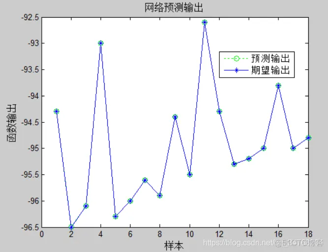
plot(test_predict,':og')
hold on
plot(test_y,'- *')
legend('预测输出','期望输出')
title('网络预测输出','fontsize',12)
ylabel('函数输出','fontsize',12)
xlabel('样本','fontsize',12)
 figure
plot(train_predict,':og')
hold on
plot(train_y,'- *')
legend('预测输出','期望输出')
title('网络预测输出','fontsize',12)
ylabel('函数输出','fontsize',12)
xlabel('样本','fontsize',12)

toc   %计算时间




【模式识别】Matlab指纹识别
【优化求解】A*算法解决三维路径规划问题
【优化求解】模拟退火遗传实现带时间窗的车辆路径规划问题
【数学建模】Matlab实现SEIR模型
【优化求解】基于NSGA-2的求解多目标柔性车间调度算法
【优化求解】蚁群算法求最优值
 【图像处理】粒子群算法结合模糊聚类分割算法实现图像的分割
【优化算法】基于粒子群算法的充电站最优布局
【优化求解】粒子群算法之电线布局优化
【优化求解】遗传算法解决背包问题
【优化求解】采用遗传算法编制多物流中心的开放式车辆路径问题Matlab程序
完整代码添加QQ1575304183