Copula-GLM——用于尖峰分析研究（Matlab代码实现）

最新推荐文章于 2025-12-19 16:12:26 发布

原创最新推荐文章于 2025-12-19 16:12:26 发布 · 55 阅读

0 ·

CC 4.0 BY-SA版权

文章标签：

#matlab #机器学习 #人工智能

本文介绍了Copula-GLM模型，一种结合Copula函数和广义线性模型的方法，用于分析随机事件间的相关性，尤其在尖峰分析中的应用。通过Matlab代码展示了模型的构建过程和参数估计，以及Granger因果性检测。

💥💥💞💞欢迎来到本博客❤️❤️💥💥

🏆博主优势：🌞🌞🌞博客内容尽量做到思维缜密，逻辑清晰，为了方便读者。

⛳️座右铭：行百里者，半于九十。

📋📋📋本文目录如下：🎁🎁🎁

目录

💥1 概述

📚2 运行结果

🎉3 参考文献

🌈4 Matlab代码实现

💥1 概述

Copula-GLM（Copula Generalized Linear Model）是一种基于Copula函数的建模方法，常用于模拟和分析随机事件之间的相关性。 Copula-GLM模型将Copula函数和GLM模型相结合，用于对神经元放电之间的相关性进行建模。

Copula-GLM是一种用于尖峰分析研究的统计模型。尖峰分析是一种用于研究极端事件的方法，例如极端气候事件或金融市场崩盘。Copula-GLM模型基于Copula函数和广义线性模型（GLM）的组合，可以用于建立联合分布函数，从而分析极端事件的概率和影响因素。

Copula函数是一种用于描述随机变量之间依赖关系的数学工具。它可以将边缘分布和相关性分离开来，从而更准确地描述随机变量之间的关系。GLM则是一种广泛使用的统计模型，可以用于建立因变量和自变量之间的关系，包括线性和非线性关系。

在Copula-GLM模型中，首先需要选择合适的Copula函数和边缘分布函数。然后，可以使用GLM建立因变量和自变量之间的关系。最终，可以使用模型来预测极端事件的概率和影响因素。

Copula-GLM模型可以用于各种领域的尖峰分析研究，例如气候变化、金融市场和风险管理等。它可以帮助研究人员更准确地了解极端事件的概率和影响因素，从而制定更有效的应对策略。

📚2 运行结果

主函数部分代码：

% Demo codes for the Copula-based Granger causality for spike train data

clear
%% Simulated data generation

% number of trials for the simulated data
Ntrial=50;

% Length of simulated data
Npoint=1000;

% copula coefficient for generating simulated data
rho=0.5;


% generate bivariate data with causal influence
% marginal regressions:
% Y1: logit(p1) = beta1 + beta2*Y1(t-1) + beta3*Y2(t-1)
% Y2: logit(p2) = beta4 + beta5*Y1(t-1) + beta6*Y2(t-1)
% 
% beta1 = 0.5
% beta2 = -0.5
% beta3 = 0
% beta4 = -2
% beta5 = 1
% beta6 = 0.5
% 
% Thus, true Granger causality is Y1 -> Y2

dat = gendata_gc(Ntrial,Npoint,rho);

% model order
porder=1;

% parameter for model estimation
options = optimset('GradObj','on','Display','off','TolFun',1e-4,'TolX',1e-4,'LargeScale','off','MaxIter',200);


%% Copula Granger causality (Frank)

gc12_frank=[];
gc21_frank=[];
para_frank=[];
for n=1:size(dat,1)
    Y1=squeeze(dat(n,:,1));
    Y2=squeeze(dat(n,:,2));
% designed Granger causality: Y1->Y2
    try
% Frank copula
        [gc12_frank(n) gc21_frank(n) para_frank(:,n)]=CopuReg_GC_Frank_fminunc(Y1,Y2,porder,options);
    end  
end

%%%%%%%%% Comparing the true and estimated parameters

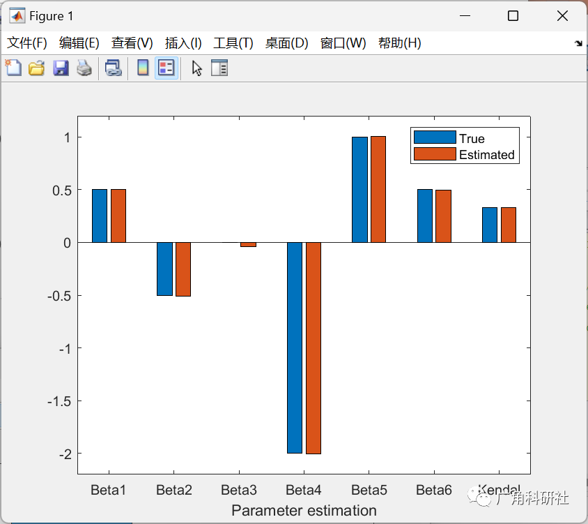
beta_est = mean(para_frank(1:6,:)');
ken_est = [];
for i = 1:Ntrial
%     rho_est=[rho_est,copulaparam('Gaussian',copulastat('Frank',para_frank(7,i)))];
    ken_est=[ken_est,copulastat('Frank',para_frank(7,i))];
end
ken_est = mean(ken_est);

para_true = [0.5 -0.5 0 -2 1 0.5 copulastat('Gaussian',0.5)];
para_est = [beta_est ken_est];

figure
bar([para_true; para_est]')
xlabel('Parameter estimation')
set(gca,'XTick',[1:7],'XTicklabel',{' Beta1 ' ' Beta2 ' ' Beta3 ' ' Beta4 ' ' Beta5 ' ' Beta6 ' 'Kendal'});
ax=axis;
axis([ax(1) ax(2) -2.2 1.2])
legend('True','Estimated')


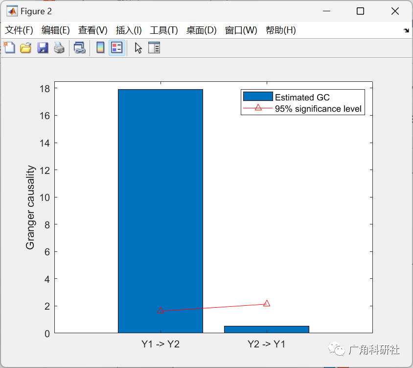
%%%%%%%%% Granger causality

dat_perm1 = cat(3,dat(randperm(Ntrial),:,1),dat(randperm(Ntrial),:,2));
dat_perm2 = cat(3,dat(randperm(Ntrial),:,1),dat(randperm(Ntrial),:,2));
dat_perm = cat(1,dat_perm1,dat_perm2);

gc12_frank_perm=[];
gc21_frank_perm=[];
for n=1:size(dat_perm,1)
    Y1_perm=squeeze(dat_perm(n,:,1));
    Y2_perm=squeeze(dat_perm(n,:,2));
% designed Granger causality: Y1->Y2
    try
% Frank copula
        [gc12_frank_perm(n) gc21_frank_perm(n)]=CopuReg_GC_Frank_fminunc(Y1_perm,Y2_perm,porder,options);
    end  
end

sig_alpha = 0.05;

gc12tmp = sort(gc12_frank_perm);
gc12_thresh = gc12tmp(fix(length(gc12tmp)*(1-sig_alpha)));
gc21tmp = sort(gc21_frank_perm);
gc21_thresh = gc21tmp(fix(length(gc21tmp)*(1-sig_alpha)));

figure;
bar([mean(gc12_frank) mean(gc21_frank)])
hold on
plot([1,2],[gc12_thresh,gc21_thresh],'color','red','marker','^')
set(gca,'XTick',[1:2],'XTicklabel',{'Y1 -> Y2' 'Y2 -> Y1'});
axis([0 3 0 18.5])
legend('Estimated GC','95% significance level')
ylabel('Granger causality')


%%  Copula Granger causality (Gaussian); Note the Gaussian code would run slower than the Frank


gc12_Gauss=[];
gc21_Gauss=[];
para_Gauss=[];
for n=1:size(dat,1)
    Y1=squeeze(dat(n,:,1));
    Y2=squeeze(dat(n,:,2));
% designed Granger causality: Y1->Y2
    try
% Frank copula
        [gc12_Gauss(n) gc21_Gauss(n) para_Gauss(:,n)]=CopuReg_GC_Gauss_fminunc(Y1,Y2,porder,options);
    end  
    
    n
end

%%%%%%%%% Comparing the true and estimated parameters

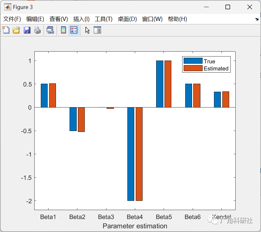
beta_est = mean(para_Gauss(1:6,:)');
ken_est = [];
for i = 1:Ntrial
%     rho_est=[rho_est,copulaparam('Gaussian',copulastat('Frank',para_frank(7,i)))];
    tmpgau = -1+2*exp(-exp(para_Gauss(7,i)));
    ken_est=[ken_est,copulastat('Gaussian',tmpgau)];
end
ken_est = mean(ken_est);

para_true = [0.5 -0.5 0 -2 1 0.5 copulastat('Gaussian',0.5)];
para_est = [beta_est ken_est];

figure
bar([para_true; para_est]')
xlabel('Parameter estimation')
set(gca,'XTick',[1:7],'XTicklabel',{' Beta1 ' ' Beta2 ' ' Beta3 ' ' Beta4 ' ' Beta5 ' ' Beta6 ' 'Kendal'});
ax=axis;
axis([ax(1) ax(2) -2.2 1.2])
legend('True','Estimated')


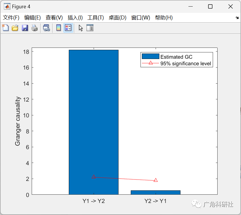
%%%%%%%%% Granger causality

dat_perm1 = cat(3,dat(randperm(Ntrial),:,1),dat(randperm(Ntrial),:,2));
dat_perm2 = cat(3,dat(randperm(Ntrial),:,1),dat(randperm(Ntrial),:,2));
dat_perm = cat(1,dat_perm1,dat_perm2);

gc12_Gauss_perm=[];
gc21_Gauss_perm=[];
for n=1:size(dat_perm,1)
    Y1_perm=squeeze(dat_perm(n,:,1));
    Y2_perm=squeeze(dat_perm(n,:,2));
% designed Granger causality: Y1->Y2
    try
% Frank copula
        [gc12_Gauss_perm(n) gc21_Gauss_perm(n)]=CopuReg_GC_Gauss_fminunc(Y1_perm,Y2_perm,porder,options);
    end  
end

sig_alpha = 0.05;

gc12tmp = sort(gc12_Gauss_perm);
gc12_thresh = gc12tmp(fix(length(gc12tmp)*(1-sig_alpha)));
gc21tmp = sort(gc21_Gauss_perm);
gc21_thresh = gc21tmp(fix(length(gc21tmp)*(1-sig_alpha)));

figure;
bar([mean(gc12_Gauss) mean(gc21_Gauss)])
hold on
plot([1,2],[gc12_thresh,gc21_thresh],'color','red','marker','^')
set(gca,'XTick',[1:2],'XTicklabel',{'Y1 -> Y2' 'Y2 -> Y1'});
axis([0 3 0 18.5])
legend('Estimated GC','95% significance level')
ylabel('Granger causality')