《机器学习》编程作业的Python实现【ex2_reg.py】

代码

import numpy as np 
import matplotlib.pyplot as plt 
import scipy.optimize as op 

def plotData(X, y):
    index0 = list()
    index1 = list()
    j = 0
    for i in y:
        if i == 0:
            index0.append(j)
        else:
            index1.append(j)
        j = j + 1
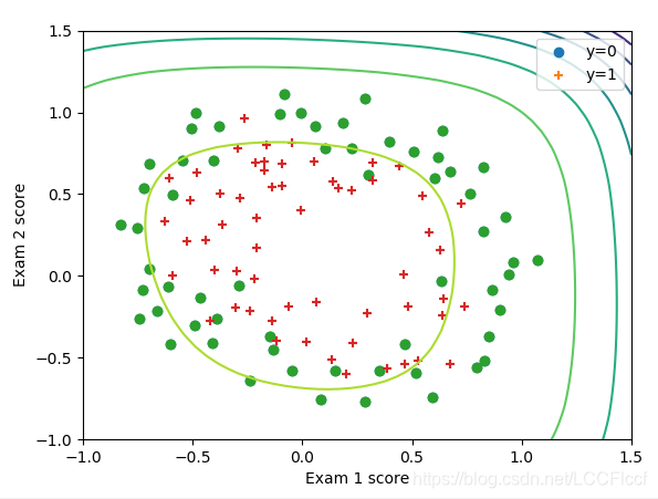
    plt.scatter(X[index0, 0], X[index0, 1], marker='o')
    plt.scatter(X[index1, 0], X[index1, 1], marker='+')
    plt.xlabel('Exam 1 score')
    plt.ylabel('Exam 2 score')
    plt.legend(['y=0', 'y=1'], loc='upper right')
    # plt.show()

def mapFeature(X1, X2):
	degree = 6
	out = np.ones((X1.shape[0], 1))
	for i in range(1, degree + 1):
		for j in range(0,i+1):
			newColum = (X1 ** (i-j))*(X2 ** j)
			out = np.column_stack((out, newColum))
	return out

def mapFeature1(x1, x2):
    degree = 6
    out = np.ones((1, 1))
    for i in range(1, degree+1):
        for j in range(0, i+1):
            newColumn = (x1 ** (i - j))*(x2 ** j)
            out = np.column_stack((out, newColumn))
    return out


def sigmoid(z):
	return 1 / (1 + np.exp(-z))

def costFunctionReg_cost(initial_theta, X, y, Lambda):
	m, n = np.shape(X)
	initial_theta = initial_theta.reshape((n,1))
	h = sigmoid(X.dot(initial_theta))
	#theta的第一个不参与正则化，需变为0
	theta_temp = initial_theta.copy()
	theta_temp[0] = 0

	#theta_temp = np.row_stack((0 ,initial_theta[1:])) #用这种方法会出BUG
	J = (1/m) * np.sum(-1*y*np.log(h) - (1-y)*np.log(1-h)) +\
			 (Lambda/(2*m)) * np.dot(theta_temp.T,theta_temp)
	return J

def costFunctionReg_grad(initial_theta, X, y, Lambda):
	m, n = np.shape(X)
	initial_theta = initial_theta.reshape((n,1))
	h = sigmoid(X.dot(initial_theta))
	theta_temp = initial_theta.copy()
	theta_temp[0] = 0
	#$theta_temp = np.row_stack((0, initial_theta[1:]))
	grad = (X.T).dot(h-y) / m + Lambda/m * theta_temp
	return grad.flatten()

def plotDecisionBoundary(theta, X, y):
    figure = plotData(X[:, 1:], y)
    m, n = X.shape
    # Only need 2 points to define a line, so choose two endpoints
    if n <= 3:
        point1 = np.min(X[:, 1])
        point2 = np.max(X[:, 1])
        point = np.array([point1, point2])
        plot_y = -1*(theta[0] + theta[1]*point)/theta[2]
        plt.plot(point, plot_y, '-')
        plt.legend(['Admitted', 'Not admitted', 'Boundary'], loc='lower left')
    else:
    	u = np.linspace(-1, 1.5, 50)
    	v = u.copy()
    	z = np.zeros((u.shape[0], v.shape[0]))
    	for i in range(u.shape[0]):
    		for j in range(v.shape[0]):
    			z[i, j] = mapFeature1(u[i], v[j]).dot(theta)
    	z = z.T
    	#print(u.shape)
    	#print(z.shape)
    	plt.contour(u, v, z)
    plt.show()
    return 0



if __name__ == '__main__':
# ======================load data========================
	file = 'ex2data2.txt'
	data = np.loadtxt(file, delimiter=',')
	X = data[:,:2]
	y = data[:,2].reshape((data.shape[0],1))
	plotData(X, y)
# =========== Part 1: Regularized Logistic Regression ============

	X = mapFeature(X[:,0], X[:,1])

# initialize fitting parameters
	initial_theta = np.zeros((X.shape[1], 1))
# set regularization parameter lambda to 1
	Lambda = 1
	cost = costFunctionReg_cost(initial_theta, X, y, Lambda)
	grad = costFunctionReg_grad(initial_theta, X, y, Lambda)
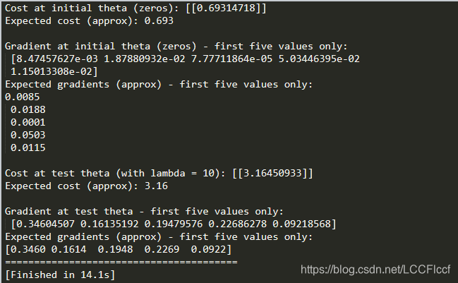
	print('Cost at initial theta (zeros):',cost)
	print('Expected cost (approx): 0.693\n')
	print('Gradient at initial theta (zeros) - first five values only:\n',grad[0:5])
	print('Expected gradients (approx) - first five values only:')
	print('0.0085\n 0.0188\n 0.0001\n 0.0503\n 0.0115\n')

# Compute and display cost and gradient with all-ones theta and lambda = 10
	Lambda = 10
	test_theta = np.ones((X.shape[1], 1))

	cost = costFunctionReg_cost(test_theta, X, y, Lambda)
	grad = costFunctionReg_grad(test_theta, X, y, Lambda)
	print('Cost at test theta (with lambda = 10):',cost)
	print('Expected cost (approx): 3.16\n')
	print('Gradient at test theta - first five values only:\n',grad[0:5])
	print('Expected gradients (approx) - first five values only:')
	print('[0.3460\t0.1614\t0.1948\t0.2269\t0.0922]')
	print('='*40)

# ============= Part 2: Regularization and Accuracies =============
#  Optional Exercise:
#  In this part, you will get to try different values of lambda and
#  see how regularization affects the decision coundart
#
#  Try the following values of lambda (0, 1, 10, 100).
#
#  How does the decision boundary change when you vary lambda? How does
#  the training set accuracy vary?

# Initialize fitting parameters
	initial_theta = np.zeros((X.shape[1], 1))
	#set the different lambda
	myLambda = 5
	#optimize

	Result = op.minimize(fun=costFunctionReg_cost, \
						 x0=initial_theta, \
						 args=(X,y,myLambda),\
						 method='TNC',\
						 jac=costFunctionReg_grad)
	theta = Result.x
	cost = Result.fun
# Plot Boundary
	plotDecisionBoundary(theta, X, y)
#  end


	

运行结果

踩到的坑

1、手误把np.ones() 和 np.zeros() 混淆
2、在处理正则化项的theta时出错：自以为是地把theta第一列全部变成0，在合并向量时检索错误（神奇的是，此时计算Lambda=1的结果正确）
                正确的做法是把theta的第一项变为0（theta为（n x 1）的列向量)
                原因：对正则化理解不透彻

3、array作为参数传入到定义的函数里时，shape可能会改变。这里遇到的坑是：
            initial_theta在设定时是(28,1)，但到了def costFunctionReg_grad()的肚子里面就变成了(28, )，
             如果不reshape一下，就会报错：“ValueError: operands could not be broadcast together with shapes (28,118) (28,) ”
            这是经常踩到的坑！！！！！