一阶滞后系统传递函数的阶跃响应`Python`表达

一阶滞后系统的定义

一阶滞后系统（First-order Lag System）是动态系统中常见的惯性环节模型，表示输出信号相对于输入信号存在时间滞后。

它的时域模型可以表示为微分方程：

$$M\dot{y}(t)+\mu y(t)=u(t)$$

将上式进行拉普拉斯变化，得其传递函数模型：

$$G(s)=\frac{1}{Ms+\mu }=\frac{\frac{1}{\mu }}{\frac{M}{\mu }s+1}$$

令$K=\frac{1}{\mu }$，$T=\frac{M}{\mu }$，其传递函数可写成如下形式：

$$G(s)=\frac{K}{Ts+1}$$

其中，$T$ 是时间常数，$K$ 是增益，又称为放大系数。时间常数$T$是决定系统响应速度的重要参数。

Python 实现基础绘图函数

from control.matlab import *
import matplotlib.pyplot as plt
import numpy as np

plt.rcParams['font.family'] ='sans-serif' # 设置字体
plt.rcParams['xtick.direction'] = 'in' # x轴刻度线方向，向内为in，向外为out，双向为inout
plt.rcParams['ytick.direction'] = 'in' # y轴刻度线方向，向内为in，向外为out，双向为inout
plt.rcParams['xtick.major.width'] = 1.0 # x轴刻度线线宽
plt.rcParams['ytick.major.width'] = 1.0 # y轴刻度线线宽
plt.rcParams['font.size'] = 10 # 字体大小
plt.rcParams['axes.linewidth'] = 1.0 # 坐标轴线宽
plt.rcParams['mathtext.default'] = 'regular'
plt.rcParams['axes.xmargin'] = '0' #'.05'
plt.rcParams['axes.ymargin'] = '0.05'
plt.rcParams['savefig.facecolor'] = 'None'
plt.rcParams['savefig.edgecolor'] = 'None'

• 绘图线型生成器

def linestyle_generator():
    linestyle = ['-', '--', '-.', ':']
    line_id = 0
    while True:
        yield linestyle[line_id]
        line_id = (line_id + 1) % len(linestyle)

• 绘图属性设置函数

def plot_set(fig_ax, *args):
    fig_ax.set_xlabel(args[0])  # 通过参数1设置x轴标签
    fig_ax.set_ylabel(args[1])  # 通过参数2设置y轴标签
    fig_ax.grid(ls=':')
    if len(args)==3:
        fig_ax.legend(loc=args[2])  # 通过参数3设置图例位置

一阶滞后系统的传递函数Python表达

• 一阶滞后系统的阶跃响应

对于传递函数$G(s)=\frac{K}{Ts+1}$，设$T=0.5$，$K=1$，其阶跃响应（step）可以通过以下代码实现。

def cross_lines(x, y, **kwargs):
    ax = plt.gca()
    ax.axhline(y, **kwargs)
    ax.axvline(x, **kwargs)
    ax.scatter(T, 0.632, **kwargs)

fig, ax = plt.subplots(figsize=(3, 2.3))

(T, K) = (0.5, 1)   # 设置时间常数和增益
P = tf([0, K], [T, 1])  # 表达一阶滞后系统
y, t = step(P, np.arange(0, 5, 0.01))   # 阶跃响应
ax.plot(t,y, color='k')

cross_lines(T, 0.632, color='k',lw=0.5) # 绘制交点
ax.annotate('$(0.5, 0.632)$', xy=(0.7, 0.5))

ax.set_xticks(np.linspace(0, 5, 6))
plot_set(ax, 't', 'y')

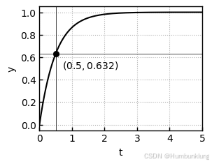
从上图可见，y值从初始值0开始不断增大，经约3秒后达到1.0。图中标注的圆点为$t=T=0.5$时的点，此时$y=0.632$。可见，实际上时间常数$T$是输出达到稳定值（经过足够长时间后的值）的63.2%时所需的时间。

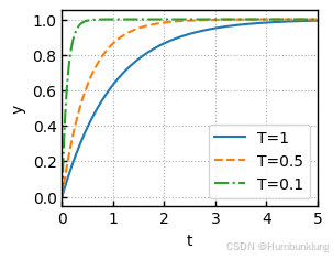
• 一阶滞后系统的阶跃响应（改变T值）

若$T\ge 0$，当$T$值改变时，系统响应也会发生变化，当增大$T$值时，系统响应会变慢，减小$T$值时，系统响应会变快。

fig, ax = plt.subplots(figsize=(3, 2.3))
LS = linestyle_generator()

K = 1
T = [1, 0.5, 0.1]   # 时间常数T分别取1，0.5和0.1
for i in range(len(T)):
    y, t = step(tf([0, K], [T[i], 1]), np.arange(0, 5, 0.01))   # 输入信号为单位阶跃
    ax.plot(t, y, ls = next(LS), label='T='+str(T[i]))


ax.set_xticks(np.linspace(0, 5, 6))
ax.set_yticks(np.linspace(0, 1, 6))
plot_set(ax, 't', 'y', 'best')

# fig.savefig("1st_step1.pdf", transparent=True, bbox_inches="tight", pad_inches=0.0)

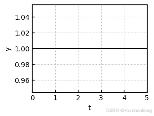
当$T=0$时，则这是一个“理想化”的无延时阶跃响应。

fig, ax = plt.subplots(figsize=(3, 2.3))

(T, K) = (0, 1)   # 设置时间常数和增益
P = tf([0, K], [T, 1])  # 表达一阶滞后系统
y, t = step(P, np.arange(0, 5, 0.01))   # 阶跃响应
ax.plot(t,y, color='k')

ax.set_xticks(np.linspace(0, 5, 6))
plot_set(ax, 't', 'y')

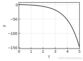
若$T<0$，其响应会发散，即不会收敛到稳定值。

fig, ax = plt.subplots(figsize=(3, 2.3))

(T, K) = (-1, 1)   # 设置时间常数和增益，T=-1
P = tf([0, K], [T, 1])  # 表达一阶滞后系统
y, t = step(P, np.arange(0, 5, 0.01))   # 阶跃响应
ax.plot(t,y, color='k')

ax.set_xticks(np.linspace(0, 5, 6))
plot_set(ax, 't', 'y')

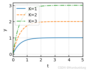
• 一阶滞后系统的阶跃响应（改变K值）

同样，改变增益$K$，我们可以看出，系统响应的阶跃响应也会改变。表现为y的稳定值发生变化，有$y(\infty )=K$。

fig, ax = plt.subplots(figsize=(3, 2.3))

LS = linestyle_generator()

T = 0.5 # 时间常数T取0.5
K = [1, 2, 3]   # 增益值K取1，2，3
for i in range(len(K)):
    y, t = step(tf([0, K[i]], [T, 1]), np.arange(0, 5, 0.01))   # 阶跃信号
    ax.plot(t,y,ls=next(LS), label='K='+str(K[i]))

ax.set_xticks(np.arange(0, 5.2, step=1.0))
ax.set_yticks(np.arange(0, 3.2, step=1))
plot_set(ax, 't', 'y', 'upper left')

# fig.savefig("1st_step2.pdf", transparent=True, bbox_inches="tight", pad_inches=0.0)