A计权的原理、算法及python 实现（需要自取）

原创于 2024-12-01 18:41:22 发布 · 2.4k 阅读

9 ·

CC 4.0 BY-SA版权

文章标签：

#算法 #机器学习 #人工智能

由于人耳对不同频率的声音的感受能力不同，即相同声压级的声音，人们会在听觉上感到不同的响度。当需要客观测量又要反映主观响度感觉的方法来度量和评估实际的声音强弱。国际标准为 IEC61672:2014

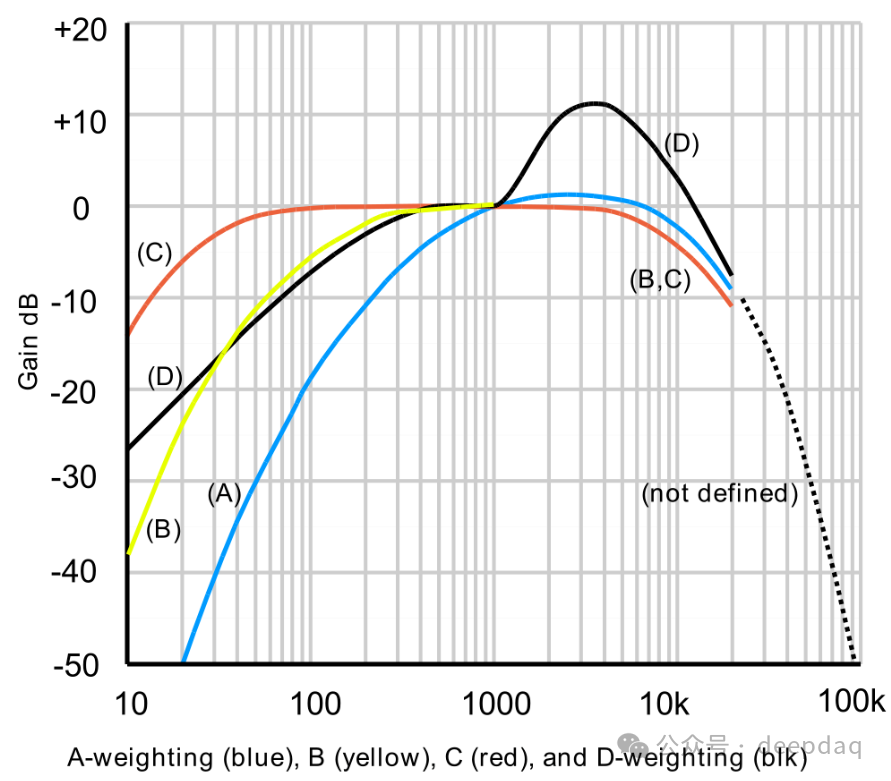
由于A计权对描述人耳听力相对于真实声学的频率响应最有意义，所以应用最为广泛。但由于A计权仅适用于相对安静的声音水平，针对噪声较大的场所譬如机场，车间等环境通常使用C计权。旧的B计权和D计权基本不再使用。

首先A计权图片是这个样子（蓝线）：

接下来就给出A-weight、C-weight曲线的解析公式：

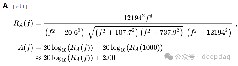
（式1）

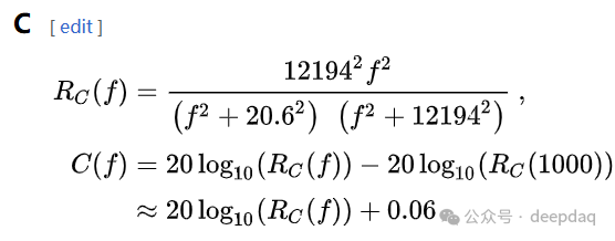
（式2）

A（f）: A-weighting to be applied, dB

C（f）: C-weighting to be applied, dB

f ：frequency, Hz；

有了上述解析公式，可以将声音进行FFT，然后利用解析式进行计算对应的A(f）、C(f)。进而进行幅值修正。但上述方法在应用范围和效率上有明显的不足。

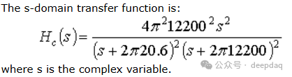
于是相关研究成果进一步的给出上述计权曲线的s 域的传递函数，在参考连接Engineering Database (archive.org)给出了如下传函：

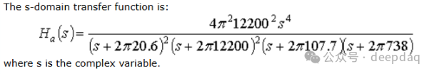
（式3）

（式4）

写到这里可以发现一个现象：一个简单的曲线可以容易的找到一个解析方程来表达，当这个解析表达式具有一个输入对应一个输出的情况时，又可以将这个解析式理解为一个简单的系统。如果这个输入是频域f时，其实这个系统就是一个滤波器而已。看来数学是对现实的抽象。（从解析式f域到s域的传递函数变换需要代入下述等式：ω=2πf ;s=jωs = j，其中j 是虚数单位），可见：如果时间域中的解析式转化为s域需要拉普拉斯变换，而频率转s域只要代入s=jω即可。

此时得到这个s域的传递函数是个模拟函数，离我们需要的z域数字滤波器还差一步：双线性变换

即将

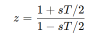
（其中，s是模拟域的复频率变量，z是数字域的复频率变量，T是采样周期）代入传递函数。得到一般式如下：

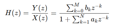
这是一阶差分方程或递推公式，其中bkb_k 和aka_k 是滤波器的系数。

上面内容我们简化为一句话：从频响函数到离散系统的变换。

来看一下设计得到的滤波器的效果：

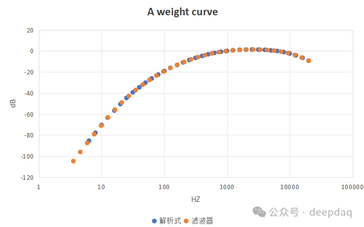
从图像对比看，滤波器实现A计权效果不错。

接下来给出相关的代码：

"""Created on Fri May 23 2014
Definitions from - ANSI S1.4-1983 Specification for Sound Level Meters, Section   5.2 Weighting Networks, pg 5. - IEC 61672-1 (2002) Electroacoustics - Sound level meters,   Part 1: Specification
"Above 20000 Hz, the relative response level shall decrease by at least 12 dBper octave for any frequency-weighting characteristic"
Appendix C:
"it has been shown that the uncertainty allowed in the A-weighted frequencyresponse in the region above 16 kHz leads to an error which may exceed theintended tolerances for the measurement of A-weighted sound level by aprecision (type 1) sound level meter.""""
import numpy as npfrom numpy import log10, pifrom scipy.signal import bilinear_zpk, freqs, sosfilt, zpk2sos, zpk2tf
__all__ = ['ABC_weighting', 'A_weighting', 'A_weight']

def ABC_weighting(curve='A'):    """    Design of an analog weighting filter with A, B, or C curve.
    Returns zeros, poles, gain of the filter.
    Examples    --------    Plot all 3 curves:
    >>> from scipy import signal    >>> import matplotlib.pyplot as plt    >>> for curve in ['A', 'B', 'C']:    ...     z, p, k = ABC_weighting(curve)    ...     w = 2*pi*np.geomspace(10, 100000, 1000)    ...     w, h = signal.freqs_zpk(z, p, k, w)    ...     plt.semilogx(w/(2*pi), 20*np.log10(h), label=curve)    >>> plt.title('Frequency response')    >>> plt.xlabel('Frequency [Hz]')    >>> plt.ylabel('Amplitude [dB]')    >>> plt.ylim(-50, 20)    >>> plt.grid(True, color='0.7', linestyle='-', which='major', axis='both')    >>> plt.grid(True, color='0.9', linestyle='-', which='minor', axis='both')    >>> plt.legend()    >>> plt.show()
    """    if curve not in 'ABC':        raise ValueError('Curve type not understood')
    # ANSI S1.4-1983 C weighting    #    2 poles on the real axis at "20.6 Hz" HPF    #    2 poles on the real axis at "12.2 kHz" LPF    #    -3 dB down points at "10^1.5 (or 31.62) Hz"    #                         "10^3.9 (or 7943) Hz"    #    # IEC 61672 specifies "10^1.5 Hz" and "10^3.9 Hz" points and formulas for    # derivation.  See _derive_coefficients()
    z = [0, 0]    p = [-2*pi*20.598997057568145,         -2*pi*20.598997057568145,         -2*pi*12194.21714799801,         -2*pi*12194.21714799801]    k = 1
    if curve == 'A':        # ANSI S1.4-1983 A weighting =        #    Same as C weighting +        #    2 poles on real axis at "107.7 and 737.9 Hz"        #        # IEC 61672 specifies cutoff of "10^2.45 Hz" and formulas for        # derivation.  See _derive_coefficients()
        p.append(-2*pi*107.65264864304628)        p.append(-2*pi*737.8622307362899)        z.append(0)        z.append(0)
    elif curve == 'B':        # ANSI S1.4-1983 B weighting        #    Same as C weighting +        #    1 pole on real axis at "10^2.2 (or 158.5) Hz"
        p.append(-2*pi*10**2.2)  # exact        z.append(0)
    # TODO: Calculate actual constants for this    # Normalize to 0 dB at 1 kHz for all curves    b, a = zpk2tf(z, p, k)    k /= abs(freqs(b, a, [2*pi*1000])[1][0])
    return np.array(z), np.array(p), k

def A_weighting(fs, output='ba'):    """    Design of a digital A-weighting filter.
    Designs a digital A-weighting filter for    sampling frequency `fs`.    Warning: fs should normally be higher than 20 kHz. For example,    fs = 48000 yields a class 1-compliant filter.
    Parameters    ----------    fs : float        Sampling frequency    output : {'ba', 'zpk', 'sos'}, optional        Type of output:  numerator/denominator ('ba'), pole-zero ('zpk'), or        second-order sections ('sos'). Default is 'ba'.
    Examples    --------    Plot frequency response
    >>> from scipy.signal import freqz    >>> import matplotlib.pyplot as plt    >>> fs = 200000    >>> b, a = A_weighting(fs)    >>> f = np.geomspace(10, fs/2, 1000)    >>> w = 2*pi * f / fs    >>> w, h = freqz(b, a, w)    >>> plt.semilogx(w*fs/(2*pi), 20*np.log10(abs(h)))    >>> plt.grid(True, color='0.7', linestyle='-', which='both', axis='both')    >>> plt.axis([10, 100e3, -50, 20])
    Since this uses the bilinear transform, frequency response around fs/2 will    be inaccurate at lower sampling rates.    """    z, p, k = ABC_weighting('A')
    # Use the bilinear transformation to get the digital filter.    z_d, p_d, k_d = bilinear_zpk(z, p, k, fs)
    if output == 'zpk':        return z_d, p_d, k_d    elif output in {'ba', 'tf'}:        return zpk2tf(z_d, p_d, k_d)    elif output == 'sos':        return zpk2sos(z_d, p_d, k_d)    else:        raise ValueError(f"'{output}' is not a valid output form.")

def A_weight(signal, fs):    """    Return the given signal after passing through a digital A-weighting filter
    signal : array_like        Input signal, with time as dimension    fs : float        Sampling frequency    """    # TODO: Upsample signal high enough that filter response meets Type 0    # limits.  A passes if fs >= 260 kHz, but not at typical audio sample    # rates. So upsample 48 kHz by 6 times to get an accurate measurement?    # TODO: Also this could just be a measurement function that doesn't    # save the whole filtered waveform.    sos = A_weighting(fs, output='sos')    return sosfilt(sos, signal)

def _derive_coefficients():    """    Calculate A- and C-weighting coefficients with equations from IEC 61672-1
    This is for reference only. The coefficients were generated with this and    then placed in ABC_weighting().    """    import sympy as sp
    # Section 5.4.6    f_r = 1000    f_L = sp.Pow(10, sp.Rational('1.5'))  # 10^1.5 Hz    f_H = sp.Pow(10, sp.Rational('3.9'))  # 10^3.9 Hz    D = sp.sympify('1/sqrt(2)')  # D^2 = 1/2
    f_A = sp.Pow(10, sp.Rational('2.45'))  # 10^2.45 Hz
    # Section 5.4.9    c = f_L**2 * f_H**2    b = (1/(1-D))*(f_r**2+(f_L**2*f_H**2)/f_r**2-D*(f_L**2+f_H**2))
    f_1 = sp.sqrt((-b - sp.sqrt(b**2 - 4*c))/2)    f_4 = sp.sqrt((-b + sp.sqrt(b**2 - 4*c))/2)
    # Section 5.4.10    f_2 = (3 - sp.sqrt(5))/2 * f_A    f_3 = (3 + sp.sqrt(5))/2 * f_A
    # Section 5.4.11    assert abs(float(f_1) - 20.60) < 0.005    assert abs(float(f_2) - 107.7) < 0.05    assert abs(float(f_3) - 737.9) < 0.05    assert abs(float(f_4) - 12194) < 0.5
    for f in ('f_1', 'f_2', 'f_3', 'f_4'):        print(f'{f} = {float(eval(f))}')
    # Section 5.4.8  Normalizations    f = 1000    C1000 = (f_4**2 * f**2)/((f**2 + f_1**2) * (f**2 + f_4**2))    A1000 = (f_4**2 * f**4)/((f**2 + f_1**2) * sp.sqrt(f**2 + f_2**2) *                             sp.sqrt(f**2 + f_3**2) * (f**2 + f_4**2))
    # Section 5.4.11    assert abs(20*log10(float(C1000)) + 0.062) < 0.0005    assert abs(20*log10(float(A1000)) + 2.000) < 0.0005
    for norm in ('C1000', 'A1000'):        print(f'{norm} = {float(eval(norm))}')

if __name__ == '__main__':    import pytest    pytest.main(['../../tests/test_ABC_weighting.py', "--capture=sys"])

感谢小伙伴的关注，后续将陆续为大家奉上数字数据处理原理及代码实现等内容....