


Datawhale干货
作者:宋志学,Datawhale成员
作者|宋志学,编辑|SwanLab
1
多头注意力机制(Multi-Head Attention,MHA)
多头注意力(Multi-Head Attention, MHA)是Transformer模型的核心机制,通过并行计算多个注意力头,使模型能够同时关注输入序列中不同位置的特征。其核心思想是将输入映射到多个子空间,分别计算注意力权重并聚合结果,从而增强模型对复杂模式的捕捉能力。
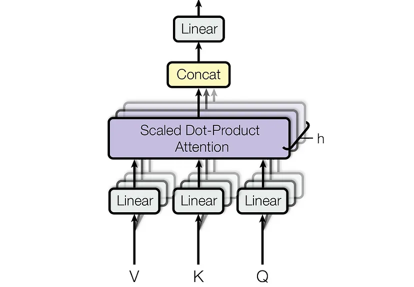
第一阶段:线性变换与多头拆分
输入序列 (批大小 ,序列长度 ,特征维度 )通过可学习参数生成查询(Query)、键(Key)、值(Value):
其中
随后,将 拆分为 个头,每个头的维度为 ,并调整形状为:
第二阶段:缩放点积注意力
每个头独立计算注意力权重:
其中 表示查询与键的相似度矩阵,缩放因子 缓解点积过大导致的梯度消失。若存在掩码(如屏蔽填充位置),则对无效位置填充。
第三阶段:多头合并与输出投影
将所有头的输出拼接并映射回原始维度:
代码实现如下:
import torchimport torch.nn as nn
class MultiHeadAttention(nn.Module):    def __init__(self, hidden_size, num_heads, dropout=0.0):        """        多头注意力机制的实现。        Args:            hidden_size (int): 输入特征的维度,也即 hidden_state 的最后一维。            num_heads (int): 注意力头的数量。            dropout (float): dropout 的概率,默认为 0.0。        """        super(MultiHeadAttention, self).__init__()
        assert hidden_size % num_heads == 0, "hidden_size 必须能被 num_heads 整除"
        self.hidden_size = hidden_size        self.num_heads = num_heads        self.head_dim = hidden_size // num_heads  # 每个头的维度
        # 定义线性变换层,用于生成 Q, K, V        self.query = nn.Linear(hidden_size, hidden_size)        self.key = nn.Linear(hidden_size, hidden_size)        self.value = nn.Linear(hidden_size, hidden_size)
        self.dropout = nn.Dropout(dropout)
        # 输出线性层        self.out_projection = nn.Linear(hidden_size, hidden_size)
    def forward(self, hidden_state, attention_mask=None):
        """        前向传播函数。        Args:            hidden_state (torch.Tensor): 输入的 hidden_state,形状为 [batch_size, seq_len, hidden_size]。            attention_mask (torch.Tensor, optional): 注意力掩码,用于屏蔽某些位置,形状为 [batch_size, seq_len]。默认为 None。        Returns:            torch.Tensor: 注意力输出,形状为 [batch_size, seq_len, hidden_size]。
        """        batch_size, seq_len, _ = hidden_state.size()
        # 1. 通过线性层得到 Q, K, V        query = self.query(hidden_state)  # [batch_size, seq_len, hidden_size]        key = self.key(hidden_state)      # [batch_size, seq_len, hidden_size]        value = self.value(hidden_state)    # [batch_size, seq_len, hidden_size]
        # 2. 将 Q, K, V 拆分成多头        query = query.view(batch_size, seq_len, self.num_heads, self.head_dim).transpose(1, 2)  # [batch_size, num_heads, seq_len, head_dim]        key = key.view(batch_size, seq_len, self.num_heads, self.head_dim).transpose(1, 2)      # [batch_size, num_heads, seq_len, head_dim]        value = value.view(batch_size, seq_len, self.num_heads, self.head_dim).transpose(1, 2)    # [batch_size, num_heads, seq_len, head_dim]
        # 3. 计算注意力权重        attention_weights = torch.matmul(query, key.transpose(-2, -1)) / (self.head_dim ** 0.5)  # [batch_size, num_heads, seq_len, seq_len]
        # 应用 attention mask        if attention_mask is not None:            attention_weights = attention_weights.masked_fill(attention_mask[:, None, None, :] == 0, float('-inf'))
        attention_weights = torch.softmax(attention_weights, dim=-1)  # [batch_size, num_heads, seq_len, seq_len]        attention_weights = self.dropout(attention_weights)
        # 4. 计算上下文向量        context = torch.matmul(attention_weights, value)  # [batch_size, num_heads, seq_len, head_dim]
        # 5. 将多头合并        context = context.transpose(1, 2).contiguous().view(batch_size, seq_len, self.hidden_size)  # [batch_size, seq_len, hidden_size]
        # 6. 通过输出线性层        output = self.out_projection(context)  # [batch_size, seq_len, hidden_size]        return outputif __name__ == '__main__':    # 示例    batch_size = 2    seq_len = 10    hidden_size = 256    num_heads = 8
    # 创建一个 MHA 实例    mha = MultiHeadAttention(hidden_size, num_heads)
    # 创建一个随机的 hidden_state    hidden_state = torch.randn(batch_size, seq_len, hidden_size)
    # 创建一个 attention mask (可选)    attention_mask = torch.ones(batch_size, seq_len)    attention_mask[:, 5:] = 0  # 屏蔽掉每个 batch 中 seq_len 的后 5 个位置
    # 通过 MHA 层    output = mha(hidden_state, attention_mask)
    # 打印输出形状    print("输出形状:", output.shape)  # torch.Size([2, 10, 256])
2
多查询注意力机制(Multi-Query Attention,MQA)
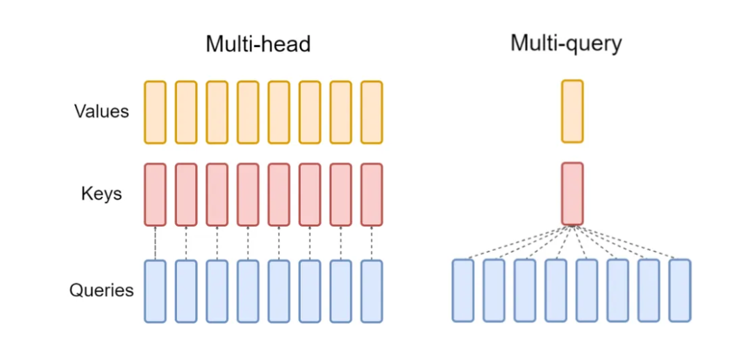
Multi-Query Attention (MQA) 是对多头注意力(MHA)的高效改进版本,其核心思想是共享键(Key)和值(Value)的投影参数,仅对查询(Query)使用独立的头参数。这种方法显著减少了模型参数量和计算复杂度,同时保留了多头注意力的部分并行性优势。
第一阶段:参数共享的线性变换
输入序列 通过以下线性变换生成 Query、共享的 Key 和 Value:
其中 是每个头独立的查询参数,而 是所有头共享的键和值参数()。与 MHA 不同,MQA 的 Key 和 Value 投影参数在头间共享,参数量减少 倍。
第二阶段:多头注意力计算
Query 被拆分为 个头(形状调整为 ),而 Key 和 Value 通过 unsqueeze 和 expand 扩展为 ,实现所有头共享相同的 Key/Value。注意力权重计算为:
(每个头独立计算)
其中 是第 个头的 Query,而 和 为共享的全局矩阵。此步骤保留了多头的并行性,但减少了 Key/Value 的冗余计算。
第三阶段:输出投影与优化
将所有头的输出拼接并通过输出投影层:
由于 Key/Value 共享,MQA 的总参数量为 ,远小于 MHA 的 (当 时)。这种设计在保持序列建模能力的同时,降低了显存占用和计算延迟,适合大规模模型部署。
代码实现如下:
import torchimport torch.nn as nnfrom thop import profile
class MultiQueryAttention(nn.Module):    def __init__(self, hidden_size, num_heads, dropout=0.0):        """        Multi-Query Attention 的实现。        Args:            hidden_size (int): 输入特征的维度,也即 hidden_state 的最后一维。            num_heads (int): 注意力头的数量。            dropout (float): dropout 的概率,默认为 0.0。        """        super(MultiQueryAttention, self).__init__()
        assert hidden_size % num_heads == 0, "hidden_size 必须能被 num_heads 整除"
        self.hidden_size = hidden_size        self.num_heads = num_heads        self.head_dim = hidden_size // num_heads  # 每个头的维度
        # 定义线性变换层,用于生成 Q, K, V        self.query = nn.Linear(hidden_size, hidden_size)  # 每个头独立的 Query        self.key = nn.Linear(hidden_size, self.head_dim)  # 所有头共享的 Key        self.value = nn.Linear(hidden_size, self.head_dim)  # 所有头共享的 Value
        self.dropout = nn.Dropout(dropout)        self.out_projection = nn.Linear(hidden_size, hidden_size)
    def forward(self, hidden_state, attention_mask=None):        """        前向传播函数。        Args:            hidden_state (torch.Tensor): 输入的 hidden_state,形状为 [batch_size, seq_len, hidden_size]。            attention_mask (torch.Tensor, optional): 注意力掩码,用于屏蔽某些位置,形状为 [batch_size, seq_len]。默认为 None。        Returns:            torch.Tensor: 注意力输出,形状为 [batch_size, seq_len, hidden_size]。        """        batch_size, seq_len, _ = hidden_state.size()
        # 1. 通过线性层得到 Q, K, V        query = self.query(hidden_state)  # [batch_size, seq_len, hidden_size]        key = self.key(hidden_state)      # [batch_size, seq_len, head_dim]        value = self.value(hidden_state)  # [batch_size, seq_len, head_dim]
        # 2. 将 Q 拆分为多头        query = query.view(batch_size, seq_len, self.num_heads, self.head_dim).transpose(1, 2)  # [batch_size, num_heads, seq_len, head_dim]
        # 3. 扩展 K 和 V 到 num_heads 维度(所有头共享相同的 K/V)        key = key.unsqueeze(1).expand(-1, self.num_heads, -1, -1)  # [batch_size, num_heads, seq_len, head_dim]        value = value.unsqueeze(1).expand(-1, self.num_heads, -1, -1)  # [batch_size, num_heads, seq_len, head_dim]
        # 4. 计算注意力权重        attention_weights = torch.matmul(query, key.transpose(-2, -1)) / (self.head_dim ** 0.5)  # [batch_size, num_heads, seq_len, seq_len]        # 应用 attention mask        if attention_mask is not None:            attention_weights = attention_weights.masked_fill(attention_mask[:, None, None, :] == 0, float('-inf'))
        attention_weights = torch.softmax(attention_weights, dim=-1)  # [batch_size, num_heads, seq_len, seq_len]        attention_weights = self.dropout(attention_weights)
        # 5. 计算上下文向量        context = torch.matmul(attention_weights, value)  # [batch_size, num_heads, seq_len, head_dim]
        # 6. 将多头合并        context = context.transpose(1, 2).contiguous().view(batch_size, seq_len, self.hidden_size)  # [batch_size, seq_len, hidden_size]
        # 7. 通过输出线性层        output = self.out_projection(context)  # [batch_size, seq_len, hidden_size]
        return output
if __name__ == '__main__':    # 示例    batch_size = 2    seq_len = 10    hidden_size = 256    num_heads = 8
    # 创建一个 MQA 实例    mqa = MultiQueryAttention(hidden_size, num_heads)
    # 创建一个随机的 hidden_state    hidden_state = torch.randn(batch_size, seq_len, hidden_size)
    # 创建一个 attention mask (可选)    attention_mask = torch.ones(batch_size, seq_len)    attention_mask[:, 5:] = 0  # 屏蔽掉每个 batch 中 seq_len 的后 5 个位置
    # 通过 MQA 层    output = mqa(hidden_state, attention_mask)
    # 打印输出形状    print("输出形状:", output.shape)  # torch.Size([2, 10, 256])
3
分组查询注意力机制(Grouped Query Attention,GQA)
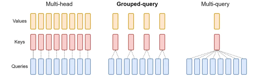
Grouped Query Attention (GQA) 是对多头注意力(MHA)和多查询注意力(MQA)的折中优化方案。其核心思想是将查询头(Query Heads)划分为多个组(Group),每组内的查询头共享一组键(Key)和值(Value),从而在保留多头并行性的同时减少参数量和计算复杂度。GQA 在参数效率与模型性能之间取得了平衡,适用于大规模模型的高效部署。
第一阶段:分组线性变换
输入序列 (批大小 ,序列长度 ,特征维度 )通过以下线性变换生成 Query、分组共享的 Key 和 Value:
其中 是每个查询头独立的参数, 为组数( 为总头数, 为每组头数), 为每个头的维度。Key 和 Value 的投影参数按组划分,每组参数共享。
第二阶段:分组注意力计算
Query 被拆分为 个头(形状调整为 ),而 Key 和 Value 被拆分为 组(每组包含 个头共享的 Key/Value)。通过 unsqueeze 和 expand 操作,将每组 Key/Value 扩展到 个头,形成 的结构。注意力权重计算为:
其中 是第 个查询头, 和 是其所属组 的共享键和值。此设计使同一组内的查询头关注相同子空间,而不同组可学习不同的特征模式。
第三阶段:输出投影与参数优化
将所有头的输出拼接并通过输出投影层:
由于每组 Key/Value 被 个头共享,GQA 的总参数量为 ,显著低于 MHA 的 (当 时)。这种设计在保持多头多样性的前提下,减少了显存占用和计算延迟,适合长序列建模和大规模模型部署。
代码实现如下:
import torchimport torch.nn as nn
class GroupedQueryAttention(nn.Module):    def __init__(self, hidden_size, num_heads, group_size=2, dropout=0.0):        """        Grouped Query Attention 实现。        Args:            hidden_size (int): 输入特征的维度。            num_heads (int): 查询头的数量。            group_size (int): 每个组中包含的查询头数量。            dropout (float): dropout 的概率。        """        super(GroupedQueryAttention, self).__init__()        assert hidden_size % num_heads == 0, "hidden_size 必须能被 num_heads 整除"        assert num_heads % group_size == 0, "num_heads 必须能被 group_size 整除"
        self.hidden_size = hidden_size        self.num_heads = num_heads        self.group_size = group_size        self.group_num = num_heads // group_size        self.head_dim = hidden_size // num_heads
        # 查询头        self.query = nn.Linear(hidden_size, hidden_size)        # 键和值头(分组共享)        self.key = nn.Linear(hidden_size, self.group_num * self.head_dim)        self.value = nn.Linear(hidden_size, self.group_num * self.head_dim)
        self.dropout = nn.Dropout(dropout)        self.out_projection = nn.Linear(hidden_size, hidden_size)
    def forward(self, hidden_state, attention_mask=None):        """        前向传播函数。        Args:            hidden_state (torch.Tensor): 输入张量,形状为 [batch_size, seq_len, hidden_size]。            attention_mask (torch.Tensor, optional): 注意力掩码,形状为 [batch_size, seq_len]。        Returns:            torch.Tensor: 注意力输出,形状为 [batch_size, seq_len, hidden_size]。        """        batch_size, seq_len, _ = hidden_state.size()
        # 1. 通过线性层生成 Q, K, V        query = self.query(hidden_state)  # [batch_size, seq_len, hidden_size]        key = self.key(hidden_state)      # [batch_size, seq_len, group_num * head_dim]        value = self.value(hidden_state)  # [batch_size, seq_len, group_num * head_dim]
        # 2. 将 Q, K, V 拆分成多头        query = query.view(batch_size, seq_len, self.num_heads, self.head_dim).transpose(1, 2)  # [batch_size, num_heads, seq_len, head_dim]
        # K 和 V 扩展到 num_heads 个头        key = key.view(batch_size, seq_len, self.group_num, self.head_dim).transpose(1, 2)  # [batch_size, group_num, seq_len, head_dim]        key = key.unsqueeze(2).expand(-1, -1, self.group_size, -1, -1).contiguous().view(batch_size, -1, seq_len, self.head_dim)  # [batch_size, num_heads, seq_len, head_dim]        value = value.view(batch_size, seq_len, self.group_num, self.head_dim).transpose(1, 2)  # [batch_size, group_num, seq_len, head_dim]        value = value.unsqueeze(2).expand(-1, -1, self.group_size, -1, -1).contiguous().view(batch_size, -1, seq_len, self.head_dim)  # [batch_size, num_heads, seq_len, head_dim]
        # 3. 计算注意力权重        attention_weights = torch.matmul(query, key.transpose(-2, -1)) / (self.head_dim ** 0.5)        if attention_mask is not None:            attention_weights = attention_weights.masked_fill(attention_mask[:, None, None, :] == 0, float('-inf'))        attention_weights = torch.softmax(attention_weights, dim=-1)        attention_weights = self.dropout(attention_weights)
        # 4. 计算上下文向量        context = torch.matmul(attention_weights, value)
        # 5. 合并多头        context = context.transpose(1, 2).contiguous().view(batch_size, seq_len, self.hidden_size)
        # 6. 输出投影        output = self.out_projection(context)        return output
# 示例if __name__ == '__main__':    batch_size = 2    seq_len = 10    hidden_size = 256    num_heads = 8    group_size = 2  # 每组 2 个头,共 4 组
    gqa = GroupedQueryAttention(hidden_size, num_heads, group_size)    hidden_state = torch.randn(batch_size, seq_len, hidden_size)    attention_mask = torch.ones(batch_size, seq_len)
    attention_mask[:, 5:] = 0  # 屏蔽后 5 个位置    output = gqa(hidden_state, attention_mask)    print("输出形状:", output.shape)  # torch.Size([2, 10, 256])
4
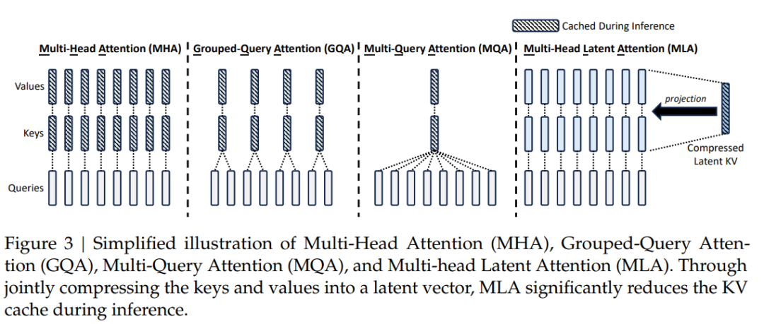
多头潜在注意力(Multi-Head Latent Attention, MLA)
Multi-Head Latent Attention (MLA) 是一种结合低秩参数化与旋转位置编码(RoPE)的高效注意力机制。其核心思想是通过低秩投影压缩查询(Q)、键(K)、值(V)的维度,并在注意力计算中解耦内容与位置信息,从而减少计算复杂度,同时保留长距离依赖建模能力。MLA 特别适用于大规模模型的部署,平衡了效率与性能。
第一阶段:低秩参数化与投影
输入序列 (批大小 ,序列长度 ,特征维度 )通过低秩投影层生成压缩的潜变量:
其中 为降维后的维度(down_dim)。随后,通过升维投影生成 Q/K/V:
此处 为升维后的维度(up_dim),低秩参数化显著减少了线性层的参数量(代码中通过 down_proj 和 up_proj 实现)。
第二阶段:解耦的内容与位置编码
MLA 将内容信息与位置信息分离处理:
内容分支:Q/K/V 的升维结果按头数 拆分为多头:
位置分支:通过 RoPE 编码增强位置感知能力:
其中 为 RoPE 的头维度(rope_head_dim),并通过 expand 操作共享至所有头(代码中通过 proj_qr 和 proj_kr 实现)。最终 Q/K 为内容与位置分支的拼接:
第三阶段:多头注意力与输出
计算注意力权重并融合内容与位置信息:
其中 直接由升维后的 生成并拆分为多头(代码中通过 v_head_dim 控制维度)。最终输出为:
MLA 的总参数量为 ,远低于传统 MHA 的 (当 时)。这种设计在保留多头多样性的前提下,显著降低了显存与计算开销。
import torchimport torch.nn as nnimport math
class RotaryEmbedding(nn.Module):    def __init__(self, hidden_size, num_heads, base=10000, max_len=512):        """        RoPE位置编码模块
        Args:            hidden_size (int): 模型维度            num_heads (int): 注意力头数量            base (int): 频率基值            max_len (int): 最大序列长度        """        super().__init__()        self.head_dim = hidden_size // num_heads        self.hidden_size = hidden_size        self.num_heads = num_heads        self.base = base        self.max_len = max_len        self.cos_pos_cache, self.sin_pos_cache = self._compute_pos_emb()
    def _compute_pos_emb(self):        theta_i = 1. / (self.base ** (torch.arange(0, self.head_dim, 2).float() / self.head_dim))        positions = torch.arange(self.max_len)        pos_emb = positions.unsqueeze(1) * theta_i.unsqueeze(0)
        cos_pos = pos_emb.sin().repeat_interleave(2, dim=-1)        sin_pos = pos_emb.cos().repeat_interleave(2, dim=-1)
        return cos_pos, sin_pos
    def forward(self, q):        """        RoPE位置编码应用
        Args:            q (torch.Tensor): 输入张量 [bs, num_heads, seq_len, head_dim]
        Returns:            torch.Tensor: 应用位置编码后的张量        """        bs, seq_len = q.shape[0], q.shape[2]        cos_pos = self.cos_pos_cache[:seq_len].to(q.device)  # [seq_len, head_dim]        sin_pos = self.sin_pos_cache[:seq_len].to(q.device)  # [seq_len, head_dim]
        # 扩展维度以匹配batch和head维度        cos_pos = cos_pos.unsqueeze(0).unsqueeze(0)  # [1, 1, seq_len, head_dim]        sin_pos = sin_pos.unsqueeze(0).unsqueeze(0)  # [1, 1, seq_len, head_dim]
        # RoPE变换        q2 = torch.stack([-q[..., 1::2], q[..., ::2]], dim=-1)  # 奇偶交替        q2 = q2.reshape(q.shape).contiguous()
        return q * cos_pos + q2 * sin_pos
class MultiHeadLatentAttention(nn.Module):    def __init__(self, hidden_size=256, down_dim=64, up_dim=128, num_heads=8, rope_head_dim=26, dropout_prob=0.0):        """        Multi-Head Latent Attention 实现
        Args:            hidden_size (int): 输入特征维度            down_dim (int): 降维后的维度            up_dim (int): 升维后的维度            num_heads (int): 注意力头数量            rope_head_dim (int): RoPE编码的头维度            dropout_prob (float): Dropout概率        """        super(MultiHeadLatentAttention, self).__init__()
        self.d_model = hidden_size        self.down_dim = down_dim        self.up_dim = up_dim        self.num_heads = num_heads        self.head_dim = hidden_size // num_heads        self.rope_head_dim = rope_head_dim        self.v_head_dim = up_dim // num_heads
        # 降维投影        self.down_proj_kv = nn.Linear(hidden_size, down_dim)        self.down_proj_q = nn.Linear(hidden_size, down_dim)
        # 升维投影        self.up_proj_k = nn.Linear(down_dim, up_dim)        self.up_proj_v = nn.Linear(down_dim, up_dim)        self.up_proj_q = nn.Linear(down_dim, up_dim)
        # 解耦Q/K投影        self.proj_qr = nn.Linear(down_dim, rope_head_dim * num_heads)        self.proj_kr = nn.Linear(hidden_size, rope_head_dim)
        # RoPE位置编码        self.rope_q = RotaryEmbedding(rope_head_dim * num_heads, num_heads)        self.rope_k = RotaryEmbedding(rope_head_dim, 1)
        # 输出层        self.dropout = nn.Dropout(dropout_prob)        self.fc = nn.Linear(num_heads * self.v_head_dim, hidden_size)        self.res_dropout = nn.Dropout(dropout_prob)
    def forward(self, h, mask=None):        """        前向传播
        Args:            h (torch.Tensor): 输入张量 [bs, seq_len, d_model]            mask (torch.Tensor): 注意力掩码 [bs, seq_len]
        Returns:            torch.Tensor: 输出张量 [bs, seq_len, d_model]        """        bs, seq_len, _ = h.size()
        # Step 1: 低秩转换        c_t_kv = self.down_proj_kv(h)  # [bs, seq_len, down_dim]        k_t_c = self.up_proj_k(c_t_kv)  # [bs, seq_len, up_dim]        v_t_c = self.up_proj_v(c_t_kv)  # [bs, seq_len, up_dim]        c_t_q = self.down_proj_q(h)  # [bs, seq_len, down_dim]        q_t_c = self.up_proj_q(c_t_q)  # [bs, seq_len, up_dim]
        # Step 2: 解耦Q/K处理        # RoPE投影处理        q_t_r = self.proj_qr(c_t_q)  # [bs, seq_len, rope_head_dim*num_heads]        q_t_r = q_t_r.view(bs, seq_len, self.num_heads, self.rope_head_dim).transpose(1, 2)  # [bs, num_heads, seq_len, rope_head_dim]        q_t_r = self.rope_q(q_t_r)  # 应用RoPE编码
        k_t_r = self.proj_kr(h)  # [bs, seq_len, rope_head_dim]        k_t_r = k_t_r.unsqueeze(1)  # [bs, 1, seq_len, rope_head_dim]        k_t_r = self.rope_k(k_t_r)  # 应用RoPE编码
        # Step 3: 注意力计算        # Q/K/V维度调整        q_t_c = q_t_c.view(bs, seq_len, self.num_heads, -1).transpose(1, 2)  # [bs, num_heads, seq_len, up_dim/num_heads]        q = torch.cat([q_t_c, q_t_r], dim=-1)  # [bs, num_heads, seq_len, (up_dim+rope_head_dim)/num_heads]
        k_t_c = k_t_c.view(bs, seq_len, self.num_heads, -1).transpose(1, 2)  # [bs, num_heads, seq_len, up_dim/num_heads]        k_t_r = k_t_r.expand(bs, self.num_heads, seq_len, -1)  # [bs, num_heads, seq_len, rope_head_dim]        k = torch.cat([k_t_c, k_t_r], dim=-1)  # [bs, num_heads, seq_len, (up_dim+rope_head_dim)/num_heads]
        # 计算注意力权重        scores = torch.matmul(q, k.transpose(-1, -2))  # [bs, num_heads, seq_len, seq_len]        scores = scores / (math.sqrt(self.head_dim) + math.sqrt(self.rope_head_dim))
        if mask is not None:            scores = scores.masked_fill(mask[:, None, None, :] == 0, float('-inf'))  # [bs, num_heads, seq_len, seq_len]
        attn_weights = torch.softmax(scores, dim=-1)  # [bs, num_heads, seq_len, seq_len]        attn_weights = self.dropout(attn_weights)
        # V维度调整        v_t_c = v_t_c.view(bs, seq_len, self.num_heads, self.v_head_dim).transpose(1, 2)  # [bs, num_heads, seq_len, v_head_dim]
        # 计算上下文向量        context = torch.matmul(attn_weights, v_t_c)  # [bs, num_heads, seq_len, v_head_dim]
        # 合并多头        context = context.transpose(1, 2).contiguous().view(bs, seq_len, -1)  # [bs, seq_len, num_heads*v_head_dim]
        # 输出投影        output = self.fc(context)  # [bs, seq_len, d_model]        output = self.res_dropout(output)
        return output
if __name__ == '__main__':    batch_size = 2    seq_len = 10    hidden_size = 256
    h = torch.randn(batch_size, seq_len, hidden_size)    mla = MultiHeadLatentAttention(hidden_size=hidden_size)
    # 创建可选掩码    mask = torch.ones(batch_size, seq_len)    mask[:, 5:] = 0
    output = mla(h, mask)    print("输出形状:", output.shape)  # 应输出 torch.Size([2, 10, 256])
Attention 计算复杂度
所有 Attention 的参数为:batch_size = 2, seq_len = 10, hidden_size = 256, num_heads = 8
========== Attention Test ==========MHA Output Shape: torch.Size([2, 10, 256])MHA Params: 263168, FLOPs: 2621440.0=======================================MQA Output Shape: torch.Size([2, 10, 256])MQA Params: 148032, FLOPs: 1474560.0=======================================GQA Output Shape: torch.Size([2, 10, 256])GQA Params: 197376, FLOPs: 1966080.0=======================================MLA Output Shape: torch.Size([2, 10, 256])MLA Params: 111082, FLOPs: 1100800.0代码如下:
import torchfrom torch import nnfrom thop import profile from contextlib import redirect_stdout
from MHA import MultiHeadAttentionfrom MQA import MultiQueryAttentionfrom GQA import GroupedQueryAttentionfrom MLA import MultiHeadLatentAttention
def count_params_and_flops(module: nn.Module, input_shape: tuple):    """    统计指定模型模块的参数量和计算量(FLOPs)    Args:        module: PyTorch 模块对象        input_shape: 输入张量的形状 (元组形式, 不包含 batch 维度)    Returns:        params_total: 总参数量        flops_total: 总计算量    """    # 构造示例输入    dummy_input = torch.randn(1, *input_shape)  # 添加 batch 维度
    # 计算参数量(单位:k)    params_total = sum(p.numel() for p in module.parameters())
    # 计算计算量(单位:GFLOPs)    with redirect_stdout(open("/dev/null", "w")):  # 屏蔽 thop 日志        flops_total, _ = profile(module, inputs=(dummy_input,))
    return params_total, flops_total
if __name__ == '__main__':    # 示例    batch_size = 2    seq_len = 10    hidden_size = 256    num_heads = 8
    # 创建一个随机的 hidden_state    hidden_state = torch.randn(batch_size, seq_len, hidden_size)
    # 创建一个 attention mask (可选)    attention_mask = torch.ones(batch_size, seq_len)    attention_mask[:, 5:] = 0  # 屏蔽掉每个 batch 中 seq_len 的后 5 个位置    print("==" * 5, " Attention  Test ", "==" * 5)    # 创建一个 MHA 实例    mha = MultiHeadAttention(hidden_size, num_heads)    # 通过 MHA 层    mha_output = mha(hidden_state, attention_mask)    # 打印输出形状    print("MHA Output Shape:", mha_output.shape)    # 统计参数量和计算量    mha_params, mha_flops = count_params_and_flops(mha, (seq_len, hidden_size))    print(f"MHA Params: {mha_params}, FLOPs: {mha_flops}")
    print("===" * 13)
    # 创建一个 MQA 实例    mqa = MultiQueryAttention(hidden_size, num_heads)    # 通过 MQA 层    mqa_output = mqa(hidden_state, attention_mask)    # 打印输出形状    print("MQA Output Shape:", mqa_output.shape)    # 统计参数量和计算量    mqa_params, mqa_flops = count_params_and_flops(mqa, (seq_len, hidden_size))    print(f"MQA Params: {mqa_params}, FLOPs: {mqa_flops}")
    print("===" * 13)
    # 创建一个 GQA 实例    group_size = 2  # 每组 2 个头,共 4 组    gqa = GroupedQueryAttention(hidden_size, num_heads, group_size)    # 通过 GQA 层    gqa_output = gqa(hidden_state, attention_mask)    # 打印输出形状    print("GQA Output Shape:", gqa_output.shape)    # 统计参数量和计算量    gqa_params, gqa_flops = count_params_and_flops(gqa, (seq_len, hidden_size))    print(f"GQA Params: {gqa_params}, FLOPs: {gqa_flops}")    print("===" * 13)    # 创建一个 MLA 实例    mla = MultiHeadLatentAttention(hidden_size=hidden_size, num_heads=num_heads)    # 通过 MLA 层    mla_output = mla(hidden_state, attention_mask)    # 打印输出形状    print("MLA Output Shape:", mla_output.shape)    # 统计参数量和计算量    mla_params, mla_flops = count_params_and_flops(mla, (seq_len, hidden_size))    print(f"MLA Params: {mla_params}, FLOPs: {mla_flops}")
参考引用
[1] 苏剑林. (2024, May). 缓存与效果的极限拉扯:从MHA、MQA、GQA到MLA.[Online]. :
https://kexue.fm/archives/10091
[2] 苏剑林. (2025, May). Transformer升级之路:20、MLA究竟好在哪里? [Online].:
https://kexue.fm/archives/10907
[3] 三重否定. 知乎文章 多头隐注意力(Multi-Head Latent Attention, MLA) 及简洁pytorch 实现:
https://zhuanlan.zhihu.com/p/715155329

一起“点赞”三连↓


 被折叠的 条评论
为什么被折叠?
被折叠的 条评论
为什么被折叠?
 到【灌水乐园】发言


