


 本文探讨了Anscombe's quartet中的四个数据集,分别计算了每个数据集中x和y的平均值、方差及相关系数,并利用statsmodels进行了线性回归分析。此外,还使用Seaborn的FacetGrid和plt.scatter进行可视化展示。
%matplotlib inline

import random

import numpy as np
import scipy as sp
import pandas as pd
import matplotlib.pyplot as plt
import seaborn as sns

import statsmodels.api as sm
import statsmodels.formula.api as smf

sns.set_context("talk")
In [4]:
anascombe = pd.read_csv('data/anscombe.csv')
anascombe.head()
Out[4]:
Part 1
For each of the four datasets...
- Compute the mean and variance of both x and y
- Compute the correlation coefficient between x and y
- Compute the linear regression line: y=β0+β1x+ϵy=β0+β1x+ϵ (hint: use statsmodels and look at the Statsmodels notebook)
# print(anascombe)
x_mean=anascombe.groupby('dataset')['x'].mean()
y_mean=anascombe.groupby('dataset')['y'].mean()
print('x_mean:',x_mean)
print('y_mean:',y_mean)

x_var=anascombe.groupby('dataset')['x'].var()
y_var=anascombe.groupby('dataset')['y'].var()
print('x_variance:',x_var)
print('y_variance:',y_var)

corr_mat=anascombe.groupby('dataset').corr()
# print(corr_mat)
print('correlation coefficient:')
print('I:',corr_mat['x']['I']['y'])
print('II:',corr_mat['x']['II']['y'])
print('III:',corr_mat['x']['III']['y'])
print('IV:',corr_mat['x']['IV']['y'])

data_group=anascombe.groupby('dataset')
indices=data_group.indices
print('the linear regression:')
for key in indices:
    group=data_group.get_group(key)
    n = len(group)
    is_train = np.random.rand(n)>-np.inf
    train = group[is_train].reset_index(drop=True)
    lin_model = smf.ols('y ~ x', train).fit()
    print('dataset '+str(key)+':')
运行结果:
x_mean: dataset
I      9.0
II     9.0
III    9.0
IV     9.0
Name: x, dtype: float64
y_mean: dataset
I      7.500909
II     7.500909
III    7.500000
IV     7.500909
Name: y, dtype: float64
x_variance: dataset
I      11.0
II     11.0
III    11.0
IV     11.0
Name: x, dtype: float64
y_variance: dataset
I      4.127269
II     4.127629
III    4.122620
IV     4.123249
Name: y, dtype: float64
correlation coefficient:
I: 0.816420516345
II: 0.816236506
III: 0.81628673949
IV: 0.816521436889
the linear regression:
dataset I:
                            OLS Regression Results
==============================================================================
Dep. Variable:                      y   R-squared:                       0.667
Model:                            OLS   Adj. R-squared:                  0.629
Method:                 Least Squares   F-statistic:                     17.99
Date:                Thu, 07 Jun 2018   Prob (F-statistic):            0.00217
Time:                        12:36:23   Log-Likelihood:                -16.841
No. Observations:                  11   AIC:                             37.68
Df Residuals:                       9   BIC:                             38.48
Df Model:                           1
Covariance Type:            nonrobust
==============================================================================
                 coef    std err          t      P>|t|      [0.025      0.975]
------------------------------------------------------------------------------
Intercept      3.0001      1.125      2.667      0.026       0.456       5.544
x              0.5001      0.118      4.241      0.002       0.233       0.767
==============================================================================
Omnibus:                        0.082   Durbin-Watson:                   3.212
Prob(Omnibus):                  0.960   Jarque-Bera (JB):                0.289
Skew:                          -0.122   Prob(JB):                        0.865
Kurtosis:                       2.244   Cond. No.                         29.1
==============================================================================

Warnings:
[1] Standard Errors assume that the covariance matrix of the errors is correctly specified.
dataset II:
                            OLS Regression Results
==============================================================================
Dep. Variable:                      y   R-squared:                       0.666
Model:                            OLS   Adj. R-squared:                  0.629
Method:                 Least Squares   F-statistic:                     17.97
Date:                Thu, 07 Jun 2018   Prob (F-statistic):            0.00218
Time:                        12:36:23   Log-Likelihood:                -16.846
No. Observations:                  11   AIC:                             37.69
Df Residuals:                       9   BIC:                             38.49
Df Model:                           1
Covariance Type:            nonrobust
==============================================================================
                 coef    std err          t      P>|t|      [0.025      0.975]
------------------------------------------------------------------------------
Intercept      3.0009      1.125      2.667      0.026       0.455       5.547
x              0.5000      0.118      4.239      0.002       0.233       0.767
==============================================================================
Omnibus:                        1.594   Durbin-Watson:                   2.188
Prob(Omnibus):                  0.451   Jarque-Bera (JB):                1.108
Skew:                          -0.567   Prob(JB):                        0.575
Kurtosis:                       1.936   Cond. No.                         29.1
==============================================================================

Warnings:
[1] Standard Errors assume that the covariance matrix of the errors is correctly specified.
dataset III:
                            OLS Regression Results
==============================================================================
Dep. Variable:                      y   R-squared:                       0.666
Model:                            OLS   Adj. R-squared:                  0.629
Method:                 Least Squares   F-statistic:                     17.97
Date:                Thu, 07 Jun 2018   Prob (F-statistic):            0.00218
Time:                        12:36:23   Log-Likelihood:                -16.838
No. Observations:                  11   AIC:                             37.68
Df Residuals:                       9   BIC:                             38.47
Df Model:                           1
Covariance Type:            nonrobust
==============================================================================
                 coef    std err          t      P>|t|      [0.025      0.975]
------------------------------------------------------------------------------
Intercept      3.0025      1.124      2.670      0.026       0.459       5.546
x              0.4997      0.118      4.239      0.002       0.233       0.766
==============================================================================
Omnibus:                       19.540   Durbin-Watson:                   2.144
Prob(Omnibus):                  0.000   Jarque-Bera (JB):               13.478
Skew:                           2.041   Prob(JB):                      0.00118
Kurtosis:                       6.571   Cond. No.                         29.1
==============================================================================

Warnings:
[1] Standard Errors assume that the covariance matrix of the errors is correctly specified.
dataset IV:
                            OLS Regression Results
==============================================================================
Dep. Variable:                      y   R-squared:                       0.667
Model:                            OLS   Adj. R-squared:                  0.630
Method:                 Least Squares   F-statistic:                     18.00
Date:                Thu, 07 Jun 2018   Prob (F-statistic):            0.00216
Time:                        12:36:23   Log-Likelihood:                -16.833
No. Observations:                  11   AIC:                             37.67
Df Residuals:                       9   BIC:                             38.46
Df Model:                           1
Covariance Type:            nonrobust
==============================================================================
                 coef    std err          t      P>|t|      [0.025      0.975]
------------------------------------------------------------------------------
Intercept      3.0017      1.124      2.671      0.026       0.459       5.544
x              0.4999      0.118      4.243      0.002       0.233       0.766
==============================================================================
Omnibus:                        0.555   Durbin-Watson:                   1.662
Prob(Omnibus):                  0.758   Jarque-Bera (JB):                0.524
Skew:                           0.010   Prob(JB):                        0.769
Kurtosis:                       1.931   Cond. No.                         29.1
==============================================================================

Warnings:
[1] Standard Errors assume that the covariance matrix of the errors is correctly specified.
Part 2
Using Seaborn, visualize all four datasets.
hint: use sns.FacetGrid combined with plt.scatter
sns.set(style='whitegrid')
g = sns.FacetGrid(anscombe, col="dataset", hue="dataset", size=3)
g.map(plt.scatter, 'x', 'y')
plt.show()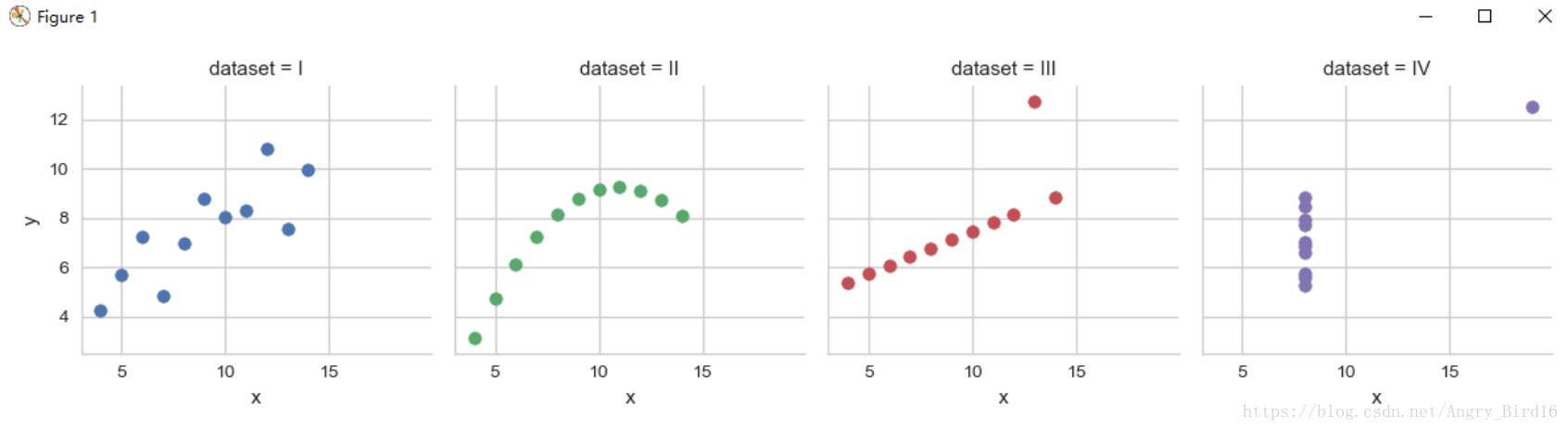


 9466
9466

 被折叠的 条评论
为什么被折叠?
被折叠的 条评论
为什么被折叠?
 到【灌水乐园】发言


