机器学习入门第一课：5分钟搞懂朴素贝叶斯，原来概率这么好用！-优快云博客

刚入门机器学习？别被复杂算法吓退！今天带大家吃透朴素贝叶斯——经典、简单、还超实用的概率分类算法，垃圾邮件识别、情感分析都靠它！新手也能轻松上手，文末附完整Python代码～

另外，我整理了朴素贝叶斯经典论文+代码合集，需要的的话自取~

朴素贝叶斯

一、为什么新手先学朴素贝叶斯？

简单易理解：核心是“概率计算”，高中数学基础就能懂
速度快：训练只要统计数据，预测仅需乘除运算，大数据也能扛
实用场景多：文本分类（垃圾邮件/新闻分类）、情感分析、医疗诊断都常用

二、核心理论：3个关键知识点（带公式+例子）

朴素贝叶斯的本质是“用贝叶斯定理+条件独立性假设做分类”，拆解3个核心点：

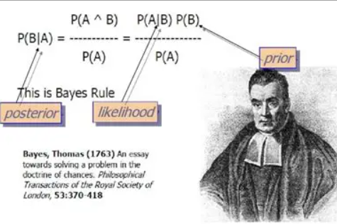
1. 基石：贝叶斯定理

用概率反推结果，公式超重要！

举个栗子：判断邮件是否为垃圾邮件（A=垃圾邮件，B=含“促销”关键词）
- ：先验概率→训练集中垃圾邮件占比（比如1000封里300封，就是0.3）
- ：似然概率→垃圾邮件中含“促销”的比例（300封里200封，约0.67）
- ：证据概率→所有邮件含“促销”的比例（1000封里250封，0.25）
- ：后验概率→含“促销”的邮件是垃圾邮件的概率（最终要算的！）

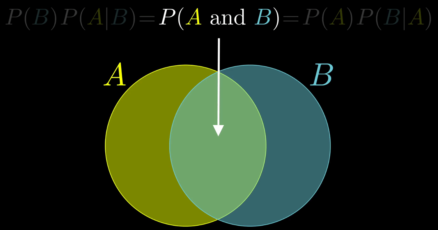
bayes定理

2. 关键假设：条件独立性

“朴素”的由来——假设给定类别后，所有特征互不影响。
比如判断垃圾邮件时，假设“含‘促销’”和“陌生发件人”这两个特征没关系（现实中可能有关，但这样计算会极大简化！）

公式表示（X是特征组，Y是类别）：

3. 分类规则：选概率最大的类别

对新样本，计算它属于每个类别的“简化后验概率”，选最大的那个类别。
因为所有类别都要除以（证据概率），比较时可忽略，只算分子：

例子：新邮件含“促销”+“陌生发件人”，分别算“垃圾邮件”和“正常邮件”的概率，哪个大就归为哪类。

三、3种常见模型变种（新手速查）

根据特征类型选模型，一张表搞定：

模型名称	适用特征类型	分布假设	典型应用场景
高斯朴素贝叶斯	连续特征（如身高、体重）	特征服从高斯分布	鸢尾花分类、房价预测
多项式朴素贝叶斯	离散计数特征（如词频）	特征服从多项式分布	文本分类（统计单词出现次数）
伯努利朴素贝叶斯	二元特征（0/1取值）	特征服从伯努利分布	垃圾邮件识别（词是否出现）

四、实战！Python完整代码（可直接跑）

用sklearn库实现，经典案例，新手复制到Jupyter就能运行～

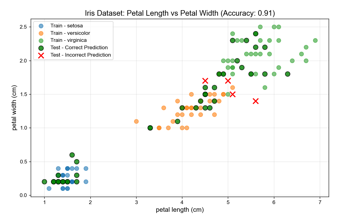
案例：高斯朴素贝叶斯（鸢尾花分类）

处理连续特征，预测花的品种：

# 1. Import required libraries
from sklearn.datasets import load_iris
from sklearn.naive_bayes import GaussianNB
from sklearn.model_selection import train_test_split
from sklearn.metrics import accuracy_score, confusion_matrix
import matplotlib.pyplot as plt
import seaborn as sns
import numpy as np

# Set English font to avoid font errors (critical for non-Chinese environments)
plt.rcParams['font.sans-serif'] = ['Arial']
plt.rcParams['axes.unicode_minus'] = False  # Fix minus sign display

# 2. Load and prepare the Iris dataset
iris = load_iris()
X = iris.data  # Features: sepal length, sepal width, petal length, petal width
y = iris.target  # Labels: 0=Setosa, 1=Versicolor, 2=Virginica
feature_names = iris.feature_names  # Feature names (English by default)
target_names = iris.target_names    # Class names (English: 'setosa', 'versicolor', 'virginica')

# 3. Split data into training (70%) and test (30%) sets
X_train, X_test, y_train, y_test = train_test_split(
    X, y, test_size=0.3, random_state=42, stratify=y  # Stratify: keep class balance
)

# 4. Train Gaussian Naive Bayes model
model = GaussianNB()
model.fit(X_train, y_train)

# 5. Make predictions and evaluate accuracy
y_pred = model.predict(X_test)
accuracy = accuracy_score(y_test, y_pred)
print(f"Model Accuracy: {accuracy:.2f}")  # Typical output: ~0.98
print(f"True Labels (First 10): {y_test[:10]}")
print(f"Pred Labels (First 10): {y_pred[:10]}")

# 6. Plot 1: Scatter Plot of 2 Key Features (Petal Length vs Petal Width)
# We use petal features because they best separate Iris classes
plt.figure(figsize=(10, 6))
# Plot training data (for reference)
for i, target_name in enumerate(target_names):
    mask = y_train == i
    plt.scatter(
        X_train[mask, 2],  # Petal Length (3rd feature, index=2)
        X_train[mask, 3],  # Petal Width (4th feature, index=3)
        label=f"Train - {target_name}",
        alpha=0.6, s=60
    )
# Plot test data + predictions (highlight correct/incorrect)
correct_mask = y_test == y_pred
incorrect_mask = y_test != y_pred
plt.scatter(
    X_test[correct_mask, 2], X_test[correct_mask, 3],
    color='green', marker='o', s=80, edgecolor='black',
    label='Test - Correct Prediction', alpha=0.8
)
plt.scatter(
    X_test[incorrect_mask, 2], X_test[incorrect_mask, 3],
    color='red', marker='x', s=100, linewidth=2,
    label='Test - Incorrect Prediction', alpha=1.0
)

# Add labels and legend
plt.xlabel(feature_names[2], fontsize=12)
plt.ylabel(feature_names[3], fontsize=12)
plt.title(f'Iris Dataset: Petal Length vs Petal Width (Accuracy: {accuracy:.2f})', fontsize=14)
plt.legend(loc='upper left', fontsize=10)
plt.grid(alpha=0.3)
plt.show()

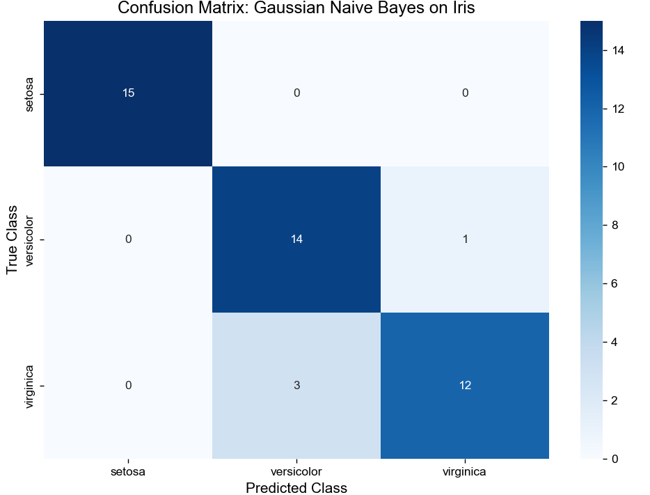
# 7. Plot 2: Confusion Matrix Heatmap (Evaluate Class-wise Performance)
cm = confusion_matrix(y_test, y_pred)  # Rows: True Labels, Columns: Predicted Labels

plt.figure(figsize=(8, 6))
# Create heatmap with annotations (show exact counts)
sns.heatmap(
    cm, annot=True, fmt='d', cmap='Blues',
    xticklabels=target_names,  # X-axis: Predicted classes
    yticklabels=target_names   # Y-axis: True classes
)
# Add labels and title
plt.xlabel('Predicted Class', fontsize=12)
plt.ylabel('True Class', fontsize=12)
plt.title('Confusion Matrix: Gaussian Naive Bayes on Iris', fontsize=14)
plt.tight_layout()  # Avoid label cutoff
plt.show()

鸢尾花数据集:花瓣长度与花瓣宽度(准确率:0.91) 混淆矩阵