Kaggle夺冠必备！一文读懂机器学习大杀器XGBoost，附完整代码与调优技巧

最新推荐文章于 2025-12-17 08:20:39 发布

原创最新推荐文章于 2025-12-17 08:20:39 发布 · 1.2k 阅读

17 ·

CC 4.0 BY-SA版权

文章标签：

#机器学习 #人工智能 #算法

机器学习算法专栏收录该内容

24 篇文章

订阅专栏

部署运行你感兴趣的模型镜像

今天和大家聊聊分类任务中常用且重要的XGBoost算法。

XGBoost

作为一种集成学习模型，它的核心是将多棵“弱”决策树组合成强预测器：不同于随机森林的并行训练与结果平均，XGBoost采用“提升”策略——树按顺序逐棵构建，每棵新树的目标都是修正前序所有树的预测误差。从直观上看，新树会去拟合当前模型的残差（严格来说是损失函数的梯度），通过这种迭代方式，持续将模型预测方向往降低损失的方向推进，最终实现精准的类别输出。

另外，我还整理了XGBOOST相关资料，需要的话可以免费分享给你

XGBoost基础详解

1. XGBoost的核心原理

XGBoost（Extreme Gradient Boosting）是一种优化的梯度提升树算法，其核心思想是通过迭代地训练弱学习器（通常是CART树）并将它们组合起来，形成一个强大的预测模型。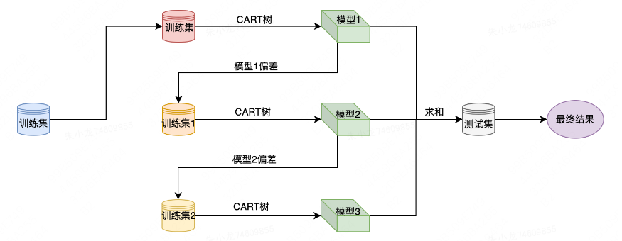算法流程图

1.1 目标函数

XGBoost的目标函数由损失函数和正则化项组成：

其中：

是损失函数，衡量预测值与真实值之间的差异
是正则化项，控制模型复杂度，防止过拟合
是树的数量

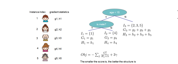
1.2 梯度提升过程

XGBoost采用加法模型，最终预测值是所有树的预测结果之和：

其中是第t轮的预测值，是第t棵树的预测结果。

每次迭代都训练一棵新树来拟合当前模型的残差（即负梯度），这就是梯度提升的核心思想。

1.3 正则化

XGBoost引入了两种主要的正则化项：

其中：

是树的叶子节点数量
是第j个叶子节点的权重
和是正则化参数

这些正则化项有助于控制树的复杂度，提高模型的泛化能力。

2. XGBoost的优势

高效性：XGBoost采用了并行计算、近似算法和缓存优化等技术，大大提高了训练速度
灵活性：支持多种目标函数，可用于分类、回归和排序等任务
鲁棒性：内置处理缺失值的机制，对异常值不敏感
可扩展性：能够处理大规模数据集

XGBoost入门项目：鸢尾花分类（完整代码、结果图和论文扫码即可免费领取）

下面我们将通过一个简单的鸢尾花分类项目来实践XGBoost的使用。

import numpy as np
import pandas as pd
import matplotlib.pyplot as plt
import seaborn as sns
from sklearn.datasets import load_iris
from sklearn.model_selection import train_test_split, GridSearchCV
from sklearn.metrics import accuracy_score, classification_report, confusion_matrix, roc_curve, auc
from sklearn.preprocessing import label_binarize
import xgboost as xgb
import os

# 设置中文字体（服务器环境可能不需要，但保持兼容性）
plt.rcParams["font.family"] = ["Arial", "Helvetica", "sans-serif"]
plt.rcParams['axes.unicode_minus'] = False  # 解决负号显示问题

# 创建结果目录
result_dir = "xgboost_iris_results"
os.makedirs(result_dir, exist_ok=True)

# 加载数据集
iris = load_iris()
X = iris.data
y = iris.target
feature_names = iris.feature_names
class_names = iris.target_names

# 数据探索
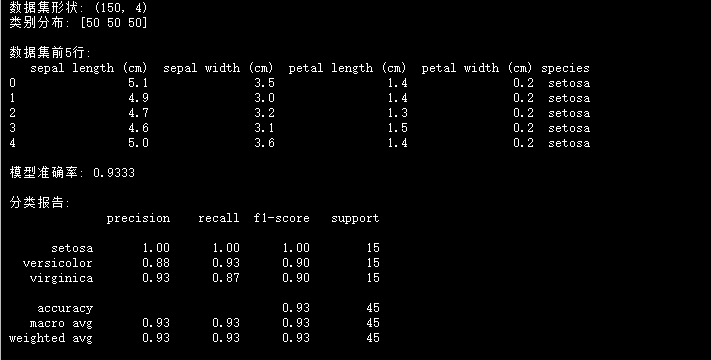
print("数据集形状:", X.shape)
print("类别分布:", np.bincount(y))

# 数据框展示前5行
df = pd.DataFrame(X, columns=feature_names)
df['species'] = [class_names[i] for i in y]
print("\n数据集前5行:")
print(df.head())

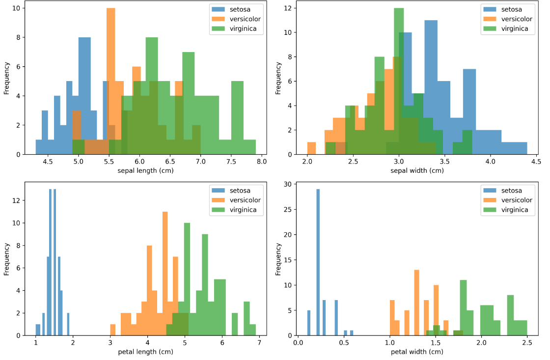
# 数据可视化 - 特征分布图
plt.figure(figsize=(12, 8))
for i, feature in enumerate(feature_names):
    plt.subplot(2, 2, i+1)
    for species in class_names:
        plt.hist(df[df['species'] == species][feature], 
                 label=species, alpha=0.7, bins=15)
    plt.xlabel(feature)
    plt.ylabel('Frequency')
    plt.legend()
plt.tight_layout()
plt.savefig(f"{result_dir}/feature_distributions.png", dpi=300, bbox_inches='tight')
plt.close()

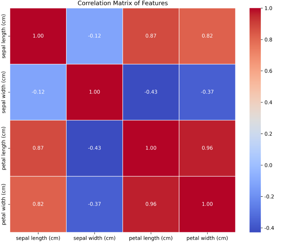
# 数据可视化 - 特征相关性热图
plt.figure(figsize=(10, 8))
corr = df.drop('species', axis=1).corr()
sns.heatmap(corr, annot=True, cmap='coolwarm', fmt=".2f", linewidths=0.5)
plt.title('Correlation Matrix of Features')
plt.savefig(f"{result_dir}/feature_correlation.png", dpi=300, bbox_inches='tight')
plt.close()

# 划分训练集和测试集
X_train, X_test, y_train, y_test = train_test_split(
    X, y, test_size=0.3, random_state=42, stratify=y
)

# 初始化XGBoost分类器
xgb_model = xgb.XGBClassifier(
    objective='multi:softmax',  # 多分类问题
    num_class=3,                # 类别数量
    random_state=42
)

# 训练模型
xgb_model.fit(X_train, y_train)

# 预测
y_pred = xgb_model.predict(X_test)
y_proba = xgb_model.predict_proba(X_test)

# 评估模型
accuracy = accuracy_score(y_test, y_pred)
print(f"\n模型准确率: {accuracy:.4f}")

print("\n分类报告:")
print(classification_report(y_test, y_pred, target_names=class_names))

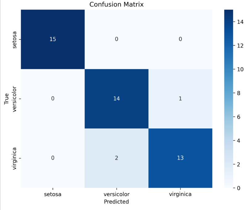
# 混淆矩阵可视化
cm = confusion_matrix(y_test, y_pred)
plt.figure(figsize=(8, 6))
sns.heatmap(cm, annot=True, fmt='d', cmap='Blues', 
            xticklabels=class_names, 
            yticklabels=class_names)
plt.xlabel('Predicted')
plt.ylabel('True')
plt.title('Confusion Matrix')
plt.savefig(f"{result_dir}/confusion_matrix.png", dpi=300, bbox_inches='tight')
plt.close()

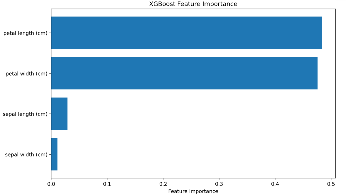
# 特征重要性可视化
feature_importance = xgb_model.feature_importances_
sorted_idx = np.argsort(feature_importance)

plt.figure(figsize=(10, 6))
plt.barh(range(len(sorted_idx)), feature_importance[sorted_idx], align='center')
plt.yticks(range(len(sorted_idx)), [feature_names[i] for i in sorted_idx])
plt.xlabel('Feature Importance')
plt.title('XGBoost Feature Importance')
plt.savefig(f"{result_dir}/feature_importance.png", dpi=300, bbox_inches='tight')
plt.close()

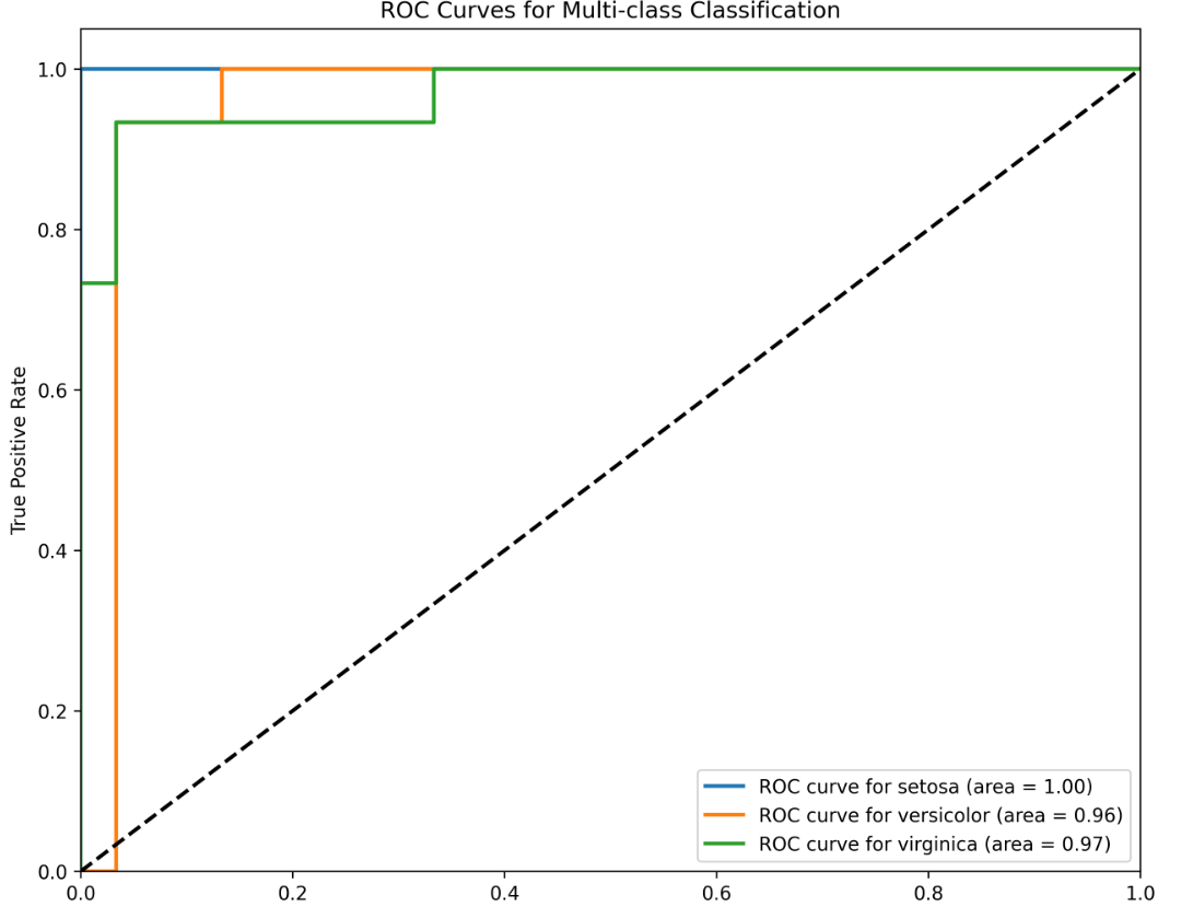
# 绘制ROC曲线（多类别的情况）
y_test_binarized = label_binarize(y_test, classes=[0, 1, 2])
n_classes = y_test_binarized.shape[1]

plt.figure(figsize=(10, 8))
for i in range(n_classes):
    fpr, tpr, _ = roc_curve(y_test_binarized[:, i], y_proba[:, i])
    roc_auc = auc(fpr, tpr)
    plt.plot(fpr, tpr, lw=2, label=f'ROC curve for {class_names[i]} (area = {roc_auc:.2f})')

plt.plot([0, 1], [0, 1], 'k--', lw=2)
plt.xlim([0.0, 1.0])
plt.ylim([0.0, 1.05])
plt.xlabel('False Positive Rate')
plt.ylabel('True Positive Rate')
plt.title('ROC Curves for Multi-class Classification')
plt.legend(loc="lower right")
plt.savefig(f"{result_dir}/roc_curves.png", dpi=300, bbox_inches='tight')
plt.close()

# 超参数调优
param_grid = {
    'max_depth': [3, 5, 7],
    'learning_rate': [0.1, 0.01, 0.001],
    'n_estimators': [100, 200, 300],
    'subsample': [0.8, 1.0]
}

grid_search = GridSearchCV(
    estimator=xgb_model,
    param_grid=param_grid,
    cv=5,
    scoring='accuracy',
    n_jobs=-1,
    verbose=1
)

grid_search.fit(X_train, y_train)

print("\n最佳参数:", grid_search.best_params_)
print("最佳交叉验证准确率:", grid_search.best_score_)

# 使用最佳参数的模型
best_model = grid_search.best_estimator_
y_pred_best = best_model.predict(X_test)
print("\n调优后模型准确率:", accuracy_score(y_test, y_pred_best))

# 保存模型
import joblib
joblib.dump(best_model, f"{result_dir}/xgboost_iris_best_model.pkl")
print(f"\n最佳模型已保存至 {result_dir}/xgboost_iris_best_model.pkl")