解构数据的七十二变：Pandas 的 Series 与 DataFrame 织梦术

原创已于 2025-04-28 00:40:07 修改 · 1.8k 阅读

20 ·

CC 4.0 BY-SA版权

文章标签：

#pandas #python #numpy

于 2025-04-26 23:57:02 首次发布

数据处理和统计分析专栏收录该内容

9 篇文章

订阅专栏

🌟 哈喽大家好，我是阳光开朗大男孩(๑•̀ㅂ•́)و✧！

🌱 学习新技能没有太晚的开始，现在就是最好的时机！

💡 注意：本文聚焦 Pandas 核心数据结构 Series 和 DataFrame 的基础用法与实战，进阶内容建议搭配官方文档食用更香～

🚀 今天带你从「0」上手 Pandas 数据处理：从环境配置到数据结构创建，再到属性方法实战，手把手教你用 Pandas 高效处理数据，为后续数据分析打下扎实基础！

👍 如果觉得干货满满，欢迎点赞收藏✨ 分享给更多正在学数据分析的小伙伴吧～

📌引言：为什么选择Pandas？四大核心优势解析

"NumPy是手术刀，Pandas是急救箱"

手术刀（NumPy）：精密的数值计算

急救箱（Pandas）：处理现实数据的全套工具

维度	NumPy数组	Pandas	优势对比
索引系统	纯数字位置索引	支持标签+位置双索引	数据定位效率提升300%
数据类型	强制统一类型	智能推断混合类型	真实数据兼容性更佳
对齐机制	无自动对齐	基于标签自动对齐	数据合并错误率降低80%
元数据	仅存储数值	支持名称/类型等属性	数据自解释性更强

一、🛠️ 环境配置与基础操作

1.1 安装指南

# Windows/Mac通用安装命令
pip install pandas

# Mac系统备用命令
pip3 install pandas

1.2 标准导入方式

import pandas as pd  # 行业标准简写

二、核心数据结构深度解析

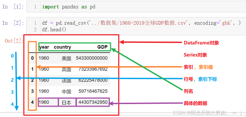
图解 Series 与 DataFrame 的结构差异

解释

DataFrame

可以把DataFrame看作由Series对象组成的字典，其中key是列名，值是Series
Series

Series和Python中的列表非常相似，但是它的每个元素的数据类型必须相同
Pandas中只有列或者二维表, 没有行的数据结构(即使是行的数据, 也会通过列的方式展示).

三、创建DataFrame的三种方式

Series是Pandas中的最基本的数据结构对象，也是DataFrame的列对象或者行对象，series本身也具有行索引。

Series是一种类似于一维数组的对象，由下面两个部分组成：

values：一组数据（numpy.ndarray类型）
index：相关的数据行索引标签；如果没有为数据指定索引，于是会自动创建一个0到N-1(N为数据的长度)的整数型索引。

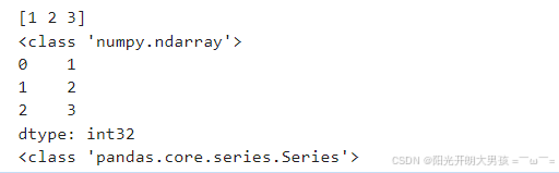
1. 自动生成索引

numpy的ndarray => Series对象

    import numpy as np
    import pandas as pd
    
    # 创建numpy.ndarray对象
    n1 = np.array([1, 2, 3])
    print(n1)
    print(type(n1))
    
    # 将上述的 ndarray对象 转成 Series对象
    s1 = pd.Series(data=n1)
    print(s1)
    print(type(s1))

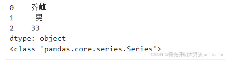
直接传入Python列表, 构建Series对象

# 这种方式可以创建Series对象, 但是没有指定 行索引值, 默认是: 0 ~ n 
# s2 = pd.Series(data=['乔峰', '男', 33]) 
s2 = pd.Series(['乔峰', '男', 33])         
# data参数名可以省略不写. print(s2) print(type(s2))     
# <class 'pandas.core.series.Series'>

3. 指定索引

传入Python列表,构建Series对象, 并指定行索引

# s3 = pd.Series(data=['乔峰', '男', 33], index=['name', 'gender', 'age'])         # data参数名可以省略不写.
s3 = pd.Series(['乔峰', '男', 33], index=['name', 'gender', 'age'])         # data参数名可以省略不写.
# s3 = pd.Series(['乔峰', '男', 33], ['name', 'gender', 'age'])         # 参数名可以省略不写.
print(s3)
print(type(s3))     # <class 'pandas.core.series.Series'>

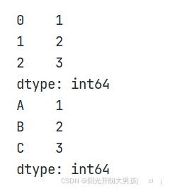
4. 通过元组和字典创建Series对象

# 使用元组
tuple1 = (1, 2, 3)
s1 = pd.Series(tuple1)
print(s1)

# 使用字典 字典中的key值是Series对象的索引值,value值是Series对象的数据值
dict1 = {'A': 1, 'B': 2, 'C': 3}
s2 = pd.Series(dict1)
print(s2)

四、构建 DataFrame 对象的实用技巧

概述

DataFrame是一个表格型的==结构化==数据结构，它含有一组或多组有序的列（Series），每列可以是不同的值类型（数值、字符串、布尔值等）。

DataFrame是Pandas中的最基本的数据结构对象，简称df；可以认为df就是一个二维数据表，这个表有行有列有索引

DataFrame是Pandas中最基本的数据结构，Series的许多属性和方法在DataFrame中也一样适用.

1. 字典方式创建

# 1. 创建字典, 记录数据.
dict_data = {
    'id': [1, 2, 3],
    'name': ['乔峰', '虚竹', '段誉'],
    'age': [33, 29, 21]
}
# 2. 基于上述的字典, 构建df对象.
# df1 = pd.DataFrame(dict_data)  
# df1 = pd.DataFrame(dict_data, index=['A', 'B', 'C'])   # 指定行索引
# index:指定行索引,  columns:指定列名(的顺序), 如果写的列名不存在, 则该列值为 NaN
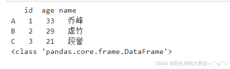
df1 = pd.DataFrame(dict_data, index=['A', 'B', 'C'], columns=['id', 'age', 'name'])   
# 3. 打印结果.
print(df1)
print(type(df1))    # <class 'pandas.core.frame.DataFrame'>

2. 列表+元组方式创建

# 1. 基于列表 + 元组, 构建数据集.  一个元组 = 一行数据
list_data = [(1, '乔峰', 33), (2, '虚竹', 29), (3, '段誉', 21)]
# 2. 构建df对象.
# df2 = pd.DataFrame(list_data, index=['X', 'Y', 'Z'], columns=['id', 'age', 'name'])  # 以行的方式传入数据, columns是设置: 列名.
df2 = pd.DataFrame(list_data, index=['X', 'Y', 'Z'], columns=['id', 'name', 'age'])  # 以行的方式传入数据, columns是设置: 列名.
# 3. 打印结果.
print(df2)
print(type(df2))

五、深度解析 Series 的常用属性

1. 常用属性介绍

属性	说明
loc	使用索引值取子集
iloc	使用索引位置取子集
dtype或dtypes	Series内容的类型
T	Series的转置矩阵
shape	数据的维数
size	Series中元素的数量
values	Series的值
index	Series的索引值

2. 代码演示

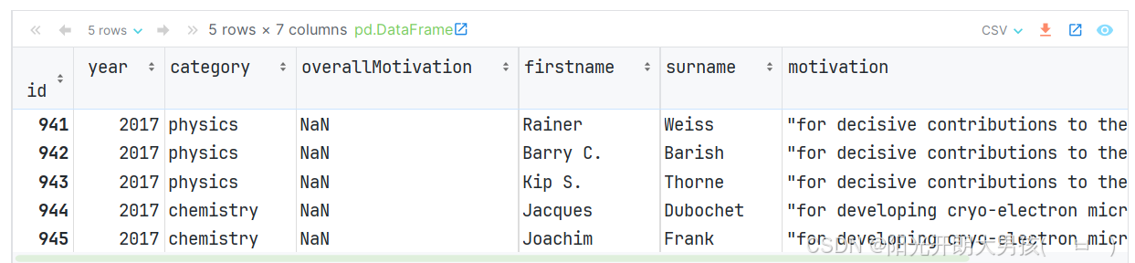
# 1. 读取 nobel_prizes.csv 文件的内容, 获取df对象. 
df = pd.read_csv('data/nobel_prizes.csv', index_col='id')   
# index_col: 设置表中的某列为 索引列. df.head()       # 默认获取前 5 条数据

（1）loc属性

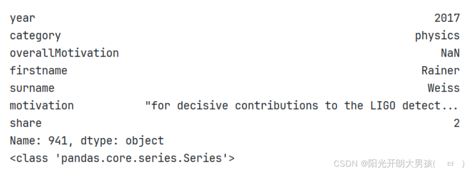
first_row = data.loc[941]
print(first_row)        # 获取第一行数据, 但是是以列的方式展示的
print(type(first_row))  # <class 'pandas.core.series.Series'>

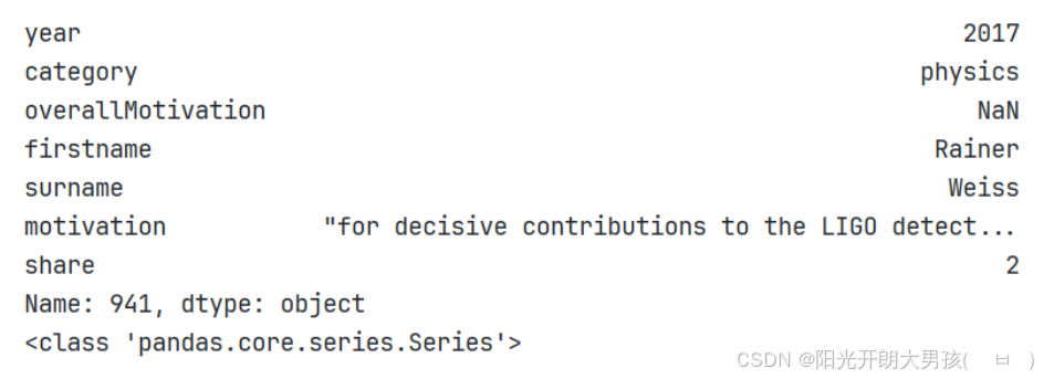
（2）iloc属性

first_row = data.iloc[0] # 使用索引位置获取自己
print(first_row)        # 获取第一行数据, 但是是以列的方式展示的
print(type(first_row))  # <class 'pandas.core.series.Series'>

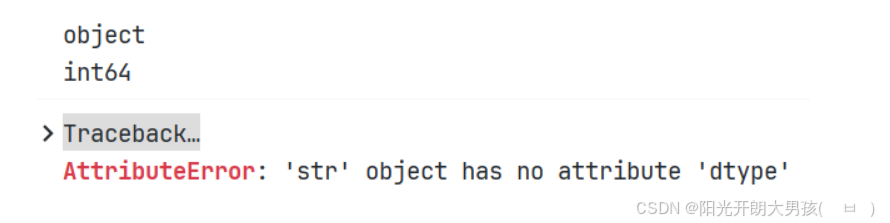
（3）dtype 或者 dtypes

print(first_row.dtype)          # 打印Series的元素类型, object表示字符串
print(first_row['year'].dtype)  # 打印Series的year列的元素类型, int64

# 打印Series的year列的元素类型, 该列值为字符串, 字符串没有dtype属性, 所以报错.
print(first_row['firstname'].dtype)

（4）shape 和 size属性

print(first_row.shape)		# 维度
# 结果为: (7,)		因为有7列元素

print(first_row.size)		# 元素个数: 7

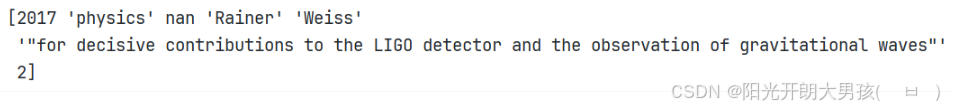
（5）values 属性

print(first_row.values) # 获取Series的元素值

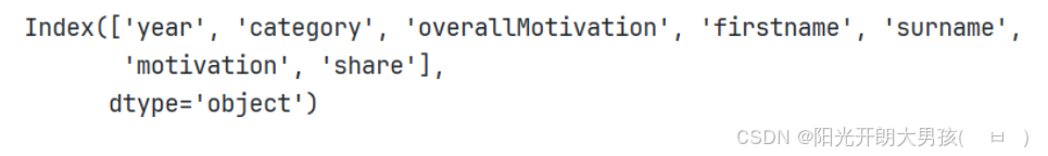
（6）index属性

print(first_row.index)  # 获取Series的索引

print(first_row.keys()) # Series对象的keys()方法, 效果同上.

六、掌握 Series 对象的实用方法

1. 常见方法

方法	说明
append	连接两个或多个Series
corr	计算与另一个Series的相关系数
cov	计算与另一个Series的协方差
describe	计算常见统计量
drop_duplicates	返回去重之后的Series
equals	判断两个Series是否相同
get_values	获取Series的值，作用与values属性相同
hist	绘制直方图
isin	Series中是否包含某些值
min	返回最小值
max	返回最大值
mean	返回算术平均值
median	返回中位数
mode	返回众数
quantile	返回指定位置的分位数
replace	用指定值代替Series中的值
sample	返回Series的随机采样值
sort_values	对值进行排序
to_frame	把Series转换为DataFrame
unique	去重返回数组
value_counts	统计不同值数量
keys	获取索引值
head	查看前5个值
tail	查看后5个值

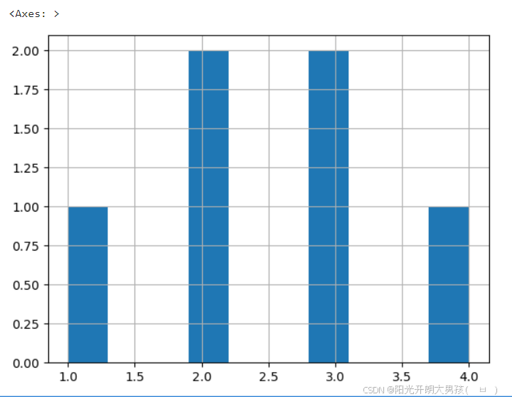
2. 代码演示

# 1. 构建Series对象.
s1 = pd.Series([1, 2, 3, 4, 2, 3], index=['A', 'B', 'C', 'D', 'E', 'F'])
print(s1)

# 2. 演示Series对象的 常用方法. 
print(len(s1))              # 长度: 6
print(s1.size)              # 长度: 6
print(s1.head())            # 默认获取前 5 条
print(s1.head(n=2))         # 指定, 获取前2条

print(s1.tail())            # 默认获取后 5条
print(s1.tail(n=3))         # 指定, 获取后3条

print(s1.keys())            # 获取Series的索引
print(s1.index)             # 获取Series的索引

print(s1.tolist())          # 转列表
print(s1.to_list())         # 效果同上
print(type(s1.tolist()))    # <class 'list'>

print(s1.to_frame())        # 转成df对象
print(type(s1.to_frame()))  # <class 'pandas.core.frame.DataFrame'>

print(s1.describe())        # 查看Series的详细信息, 例如: 最大值, 最小值, 平均值, 标准差等...
print(s1.max())
print(s1.min())
print(s1.mean())
print(s1.std())             # 标准差

print(s1.drop_duplicates()) # 去重, 返回Series对象
print(s1.unique())          # 去重, 返回数组, <class 'numpy.ndarray'>

print(s1.sort_values())                    # 根据 值 排序, 默认: 升序(ascending=True)
print(s1.sort_values(ascending=False))     # 根据 值 排序, 降序

print(s1.sort_index())                     # 根据 索引 排序, 默认: 升序
print(s1.sort_index(ascending=False))      # 根据 索引 排序, 降序

print(s1.value_counts())                   # 统计每个值出现的次数, 类似于: SQL的 group by + count()
s1.hist()                                  # 绘制: 直方图(柱状图)

七、电影数据分析实战

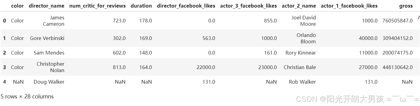
# 1. 加载数据源, 获取df对象. 
movie_df = pd.read_csv('data/movie.csv') 
movie_df.head()

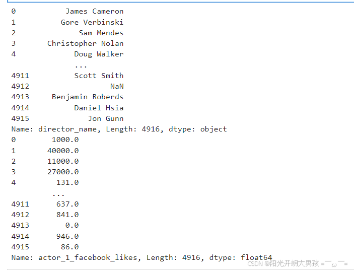
# 2. 从df对象中, 获取到 Seires对象. 
# direcctor = movie_df.director_name    # 获取: 导演名字 
direcctor = movie_df['director_name']   # 效果同上.  
print(direcctor)
         
 actor_1_fb_likes = movie_df.actor_1_facebook_likes      # 获取主演的facebook点赞数 
print(actor_1_fb_likes)

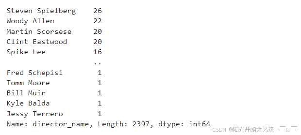
# 3. 统计不同导演指导的电影数量, 即: 各导演的总数.  
direcctor.value_counts() 
# 4. 统计主演各个点赞数 数量. 即: 1000点赞有几个, 10000点赞有几个 
# actor_1_fb_likes.value_counts()

# 5. 统计有多少空值.  
# direcctor.count()       # 4814, 统计所有的非空值 
# direcctor.shape         # (4916, ), 总量 
len(direcctor.shape)      # 4916

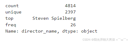
# 6. 打印描述信息 
# 查看描述信息, 例如: 最大值, 最小值, 平均值, 标准差...     
actor_1_fb_likes.describe()       
# 查看描述信息, 因为是: object(字符串类型), 所以信息没那么多.
direcctor.describe()

整合

# 加载电影数据
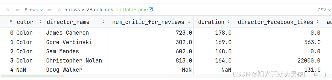
movie = pd.read_csv('data/movie.csv')   
movie.head()

# 获取 导演名(列)
director = movie.director_name      # 导演名
director = movie['director_name']   # 导演名, 效果同上
director

# 获取 主演在脸书的点赞数(列)
actor_1_fb_likes = movie.actor_1_facebook_likes # 主演在脸书的点赞数
actor_1_fb_likes.head()

# 统计相关
director.value_counts() # 不同导演的 电影数
director.count()        # 统计非空值(即: 有导演名的电影, 共有多少),  4814 
director.shape          # 总数(包括null值), (4916,)

# 查看详情
actor_1_fb_likes.describe() # 显示主演在脸书点击量的详细信息: 总数,平均值,方差等...
director.describe()         # 因为是字符串, 只显示部分统计信息

八、Series 布尔索引：精准筛选数据

从scientists.csv数据集中，列出大于Age列的平均值的具体值，具体步骤如下：

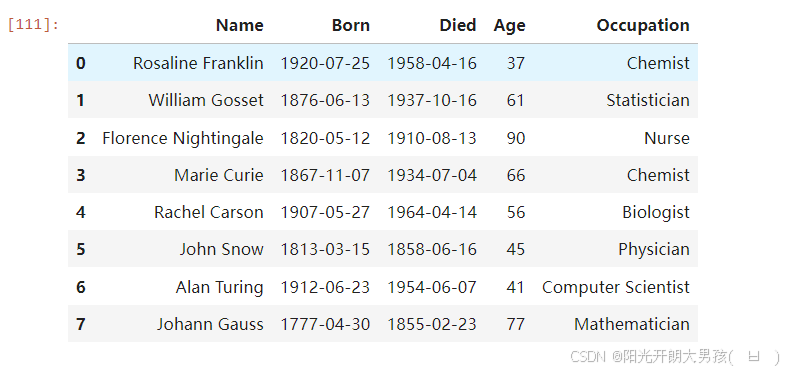
1. 加载并观察数据集

import pandas as pd

df = pd.read_csv('data/scientists.csv')
print(df)
# print(df.head())
# 输出结果如下
                   Name        Born        Died  Age          Occupation
0     Rosaline Franklin  1920-07-25  1958-04-16   37             Chemist
1        William Gosset  1876-06-13  1937-10-16   61        Statistician
2  Florence Nightingale  1820-05-12  1910-08-13   90               Nurse
3           Marie Curie  1867-11-07  1934-07-04   66             Chemist
4         Rachel Carson  1907-05-27  1964-04-14   56           Biologist
5             John Snow  1813-03-15  1858-06-16   45           Physician
6           Alan Turing  1912-06-23  1954-06-07   41  Computer Scientist
7          Johann Gauss  1777-04-30  1855-02-23   77       Mathematicia

# 演示下, 如何通过布尔值获取元素.
bool_values = [False, True, True, False, False, False, True, False]
df[bool_values]

# 输出结果如下
                   Name        Born        Died  Age          Occupation
1        William Gosset  1876-06-13  1937-10-16   61        Statistician
2  Florence Nightingale  1820-05-12  1910-08-13   90               Nurse
6           Alan Turing  1912-06-23  1954-06-07   41  Computer Scientist

2. 基于条件的筛选

计算Age列的平均值

# 获取一列数据 df[列名]
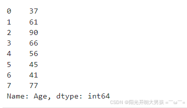
ages = df['Age']
print(ages)
print(type(ages))
print(ages.mean())

# 输出结果如下
0    37
1    61
2    90
3    66
4    56
5    45
6    41
7    77
Name: Age, dtype: int64
<class 'pandas.core.series.Series'>
59.125

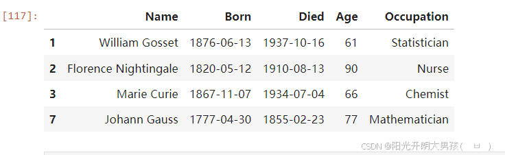
输出大于Age列的平均值的具体值

print(ages[ages > ages.mean()])

# 输出结果如下
1    61
2    90
3    66
7    77
Name: Age, dtype: int64

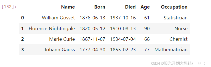
3. 布尔数组直接筛选

# 上述格式, 可以用一行代码搞定, 具体如下
df[ages > avg_age]                  # 筛选(活的)年龄 大于 平均年龄的科学家信息
df[df['Age'] > df.Age.mean()]       # 合并版写法.

九、Series 的运算规则与应用

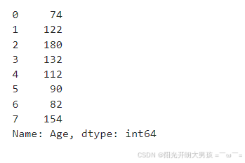
Series和数值型变量计算时，变量会与Series中的每个元素逐一进行计算；

两个Series之间计算时，索引值相同的元素之间会进行计算；索引值不同的元素的计算结果会用NaN值(缺失值)填充。

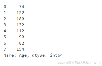
Series和数值运算, 数值会和Series的每个值进行运算.

ages_series + 10
ages_series * 2

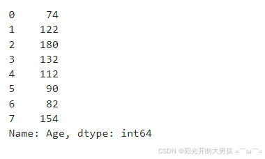
两个Series之间计算, 如果长度一致, 会按照对应的元素进行逐个计算

ages_series + ages_series

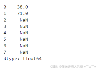
两个Series之间计算, 如果长度不一致, 则对应元素计算, 不匹配的元素用NaN填充

ages_series + pd.Series([1, 10])

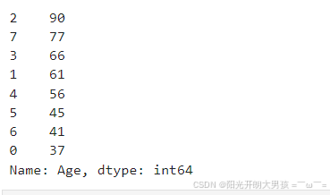
Series之间进行计算, 会尽可能依据索引来计算, 即: 优先计算索引一样的数据.

# 1. 对 源数据(ages_series), 按照 年龄 降序排列, 获取新的Series对象.
rev_series = ages_series.sort_values(ascending=False)
rev_series

# 2. 查看原始Series对象
ages_series

# 3. 具体的计算过程 
ages_series + rev_series

十、DataFrame常用属性和方法

1. 基础演示

import pandas as pd

# 加载数据集, 得到df对象
df = pd.read_csv('data/scientists.csv')

print('=============== 常用属性 ===============')
# 查看维度, 返回元组类型 -> (行数, 列数), 元素个数代表维度数
print(df.shape)
# 查看数据值个数, 行数*列数, NaN值也算
print(df.size)
# 查看数据值, 返回numpy的ndarray类型
print(df.values)
# 查看维度数
print(df.ndim)
# 返回列名和列数据类型
print(df.dtypes)
# 查看索引值, 返回索引值对象
print(df.index)
# 查看列名, 返回列名对象
print(df.columns)
print('=============== 常用方法 ===============')
# 查看前5行数据
print(df.head())
# 查看后5行数据
print(df.tail())
# 查看df的基本信息
df.info()
# 查看df对象中所有数值列的描述统计信息
print(df.describe())
# 查看df对象中所有非数值列的描述统计信息
# exclude:不包含指定类型列
print(df.describe(exclude=['int', 'float']))
# 查看df对象中所有列的描述统计信息
# include:包含指定类型列, all代表所有类型
print(df.describe(include='all'))
# 查看df的行数
print(len(df))
# 查看df各列的最小值
print(df.min())
# 查看df各列的非空值个数
print(df.count())
# 查看df数值列的平均值
print(df.mean())

2. DataFrame的布尔索引

# 小案例, 同上, 主演脸书点赞量 > 主演脸书平均点赞量的
movie[movie['actor_1_facebook_likes'] > movie['actor_1_facebook_likes'].mean()]

# df也支持索引操作
movie.head()[[True, True, False, True, False]]

3. DataFrame的计算

scientists * 2					# 每个元素, 分别和数值运算
scientists + scientists			# 根据索引进行对应运算
scientists + scientists[:4]		# 根据索引进行对应运算, 索引不匹配, 返回NAN

十一、更改Series和DataFrame对象的行索引, 列名

Pandas中99%关于DF和Series调整的API, 都会默认在副本上进行修改, 调用修改的方法后, 会把这个副本返回

这类API都有一个共同的参数: inplace, 默认值是False

如果把inplace的值改为True, 就会直接修改原来的数据, 此时这个方法就没有返回值了

1. 设置索引

（1）读取文件后, 设置行索引

# 1. 读取数据源文件, 获取 df对象
movie = pd.read_csv('data/movie.csv')
movie.head()

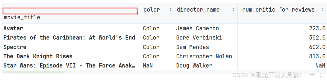
# 2. 设置 movie_tiltle(电影名) 为 行索引
# 在Pandas中, 90%以上的函数, 都是在源数据拷贝一份进行修改, 并返回副本. 而这类函数都有一个特点, 即: 有 inplace参数. 
# 默认 inplace=False, 即: 返回副本, 不修改源数据.   如果inplace=True, 则是直接修改 源数据.
# new_movie = movie.set_index('movie_title')
# new_movie.head()

movie.set_index('movie_title', inplace=True)

# 3. 查看设置后的 movie这个df对象.
movie.head()

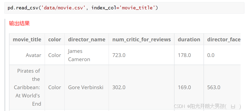
（2）读取文件时, 设置行索引

# 1. 读取数据源文件, 获取 df对象, 指定 电影名为 行索引
movie2 = pd.read_csv('data/movie.csv', index_col='movie_title')
movie2.head()

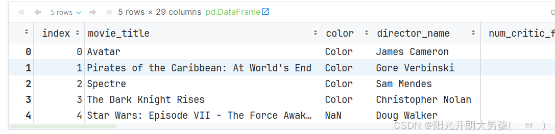
（3）通过reset_index()函数, 可以重置索引

movie2.reset_index(inplace=True)  # 取消设置的 行索引
movie2.head()

2. 修改行索引和列名

# 1. 读取数据源文件, 获取 df对象, 指定 电影名为 行索引
movie = pd.read_csv('data/movie.csv', index_col='movie_title')
movie.head()

（1）rename()函数直接修改

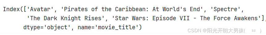
# 2. 获取 前5个列名, 方便稍后修改.
# ['Avatar', 'Pirates of the Caribbean: At World's End', 'Spectre', 'The Dark Knight Rises', 'Star Wars: Episode VII - The Force Awakens']
movie.index[:5]

# 3. 获取 前5个行索引值, 方便稍后修改.
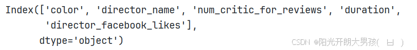
movie.columns[:5]  # ['color', 'director_name', 'num_critic_for_reviews', 'duration', 'director_facebook_likes']

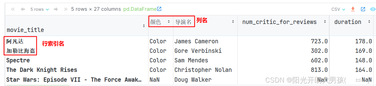
# 4. 具体的修改 列名 和 行索引的动作.
idx_name = {'Avatar': '阿凡达', "Pirates of the Caribbean: At World's End": '加勒比海盗: 直到世界尽头'}
col_name = {'color': '颜色', 'director_name': '导演名'}

movie.rename(index=idx_name, columns=col_name, inplace=True)

# 5. 查看修改后的数据
movie.head()

（2）将 index 和 column属性提取出来, 修改之后, 再放回去

# 1. 从 df中获取 行索引 和 列名的信息, 并转成列表.
idx_list = movie.index.tolist()  # 行索引信息, ['Avatar', "Pirates of the Caribbean: At World's End", 'Spectre', ...]       
col_list = movie.columns.tolist()  # 列名, ['color', 'director_name', 'num_critic_for_reviews', ...]

# 2. 修改上述的 列表(即: 行索引, 列名)信息.
idx_list[0] = '阿凡达'
idx_list[2] = '007幽灵'

col_list[0] = '颜色'
col_list[1] = '导演名'

# 3. 把上述修改后的内容, 当做新的 行索引 和 列名. 
movie.index = idx_list
movie.columns = col_list

# 4. 查看结果.
movie.head()

3. 添加, 删除, 插入列

（1）添加列

# 1. 添加列, 格式为: df['列名'] = 列值
# 新增1列, has_seen = 0, 表示是否看过这个电影. 0: 没看过, 1:看过
movie['has_seen'] = 0

# 新增1列, 总点赞量 = 导演 + 演员的 脸书点赞量
movie['director_actor_facebook_likes'] = movie['director_facebook_likes'] + movie['actor_3_facebook_likes'] + movie[
    'actor_2_facebook_likes'] + movie['actor_1_facebook_likes']

# 2. 查看结果.
movie.head()

（2）删除列或者行

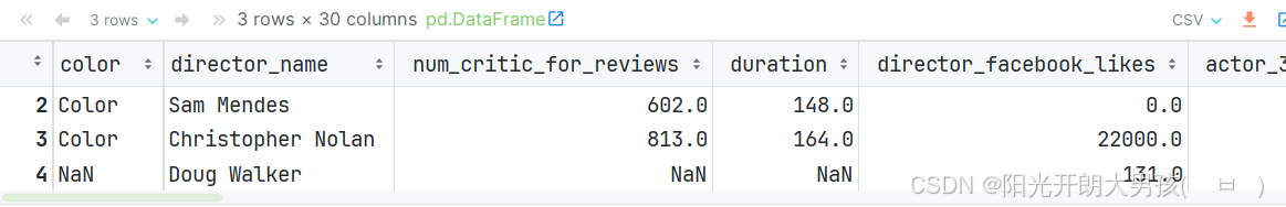
# movie.drop('has_seen')  # 报错, 需要指定方式, 按行删, 还是按列删.
# movie.drop('has_seen', axis='columns')    # 按列删
# movie.drop('has_seen', axis=1)            # 按列删, 这里的1表示: 列

movie.head().drop([0, 1])                # 按行索引删, 即: 删除索引为0和1的行

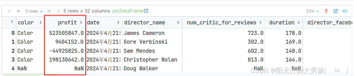
（3）插入列

有点特殊, 没有inplace参数, 默认就是在原始df对象上做插入的.

# insert() 表示插入列.   参数解释: loc:插入位置(从索引0开始计数), column=列名, value=值
# 总利润 = 总收入 - 总预算
movie.insert(loc=1, column='profit', value=movie['gross'] - movie['budget'])
movie.head()

十二、导入和导出数据

1. 读取数据

# 需求: 导出数据到 /root/output/...
# 细节: 要导出到的目的地目录, 必须存在, 即:  output目录必须存在.
# 格式:  df.to_后缀名(路径)
# 1. 准备原始df对象.
df = pd.read_csv('data/scientists.csv')
df

2. 处理数据

# 2. 对上述的df做操作, 模拟: 实际开发中, 对df对象做处理. 
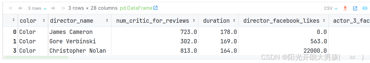
# 需求: 筛选出 年龄 大于 平均年龄的数据.
new_df = df[df.Age > df.Age.mean()]
new_df

3. 导出数据

# 3. 把上述的df对象, 写出到目的地中. 
# pickle: 比较适合 存储中间的df数据, 即: 后续要频繁使用的df对象, 可以存储下来. 
# new_df.to_pickle('output/scientists_pickle.pkl')      # pickle文件的后缀名可以是: .p, .pkl, .pickle

# excel, csv等文件, 适合于: 存储最终结果. 
# 注意: 有三个包需要安装一下, 如果你读写excel文件, 但如果你用的是Anaconda, 已经有了, 无需安装.
# new_df.to_excel('output/scientists.xls')                                 # 会把索引列也当做数据, 写出. 
# new_df.to_excel('output/scientists_noindex.xls', index=False, sheet_name='ai20')   # 不导出索引列, 且设置表名. 

# csv(用逗号隔开), tsv(用\t隔开), 适用于 数据共享, 整合等操作. 
# new_df.to_csv('output/scientists.csv')                        # 会把索引列也当做数据, 写出. 
# new_df.to_csv('output/scientists_noindex.csv', index=False)     # 不导出索引列

# 如果每行数据的 各列值之间用逗号隔开是 csv, 用\t隔开是 tsv
new_df.to_csv('output/scientists_noindex.tsv', index=False, sep='\t')     # 不导出索引列

print('导出成功!')

4. 导入数据

# 演示导入

# pickle文件
# pd.read_pickle('output/scientists_pickle.pkl') 

# excel文件
# pd.read_excel('output/scientists.xls')              # 多一列
# pd.read_excel('output/scientists_noindex.xls')      # 正常

# csv文件
# pd.read_csv('output/scientists.csv')                  # 多一列
# pd.read_csv('output/scientists_noindex.csv')          # 正常

pd.read_csv('output/scientists_noindex.tsv', sep='\t')  # 正常