week 2——Linear Regression

最新推荐文章于 2025-05-01 11:41:26 发布

三つ叶

最新推荐文章于 2025-05-01 11:41:26 发布

阅读量91

点赞数

分类专栏： Coursera机器学习文章标签：机器学习

本文链接：https://blog.youkuaiyun.com/zzhhjjjj/article/details/120707406

版权

Coursera机器学习专栏收录该内容

13 篇文章

订阅专栏

本文介绍了机器学习中的基本概念，包括训练样例的表示、预测函数和损失函数的定义，以及梯度下降法和正规方程法这两种优化策略。通过实例展示了如何在MATLAB中实现数据预处理、损失函数计算和梯度下降法更新参数的过程，同时也探讨了两种优化方法的对比和应用。

摘要生成于 C知道，由 DeepSeek-R1 满血版支持，前往体验 >

对数据表示做一些规定

$x_j^{(i)} = value\ of\ feature\ j\ in\ the\ i^{th}\ training\ example \\ x^{i} = the\ input\ (feature)\ of\ the\ i^{th}\ training\ example \\ m = the\ number\ of\ training\ examples \\ n = the\ number\ of\ features \\$

预测函数，损失函数表示

$\ function:\ h_{\theta}(x) = \theta_0+ \theta_1x_1+ \theta_2x_2+\cdots+ \theta_nx_n$
$\ function: \ J(\theta) = \frac{1}{2m}\sum\limits_{i=1}^{m}(h_\theta(x_i)-y_i)^2$

梯度下降法

repeat until convergence：{ $\\ \theta_j = \theta_j - \alpha\frac{\partial J(\theta)}{\partial\theta_j} = \theta_j - \alpha\frac{1}{m}\sum\limits_{i=1}^{m}((h_\theta(x^{(i)}) - y^{(i)})x_j^{(i)})$
}

数据归一化

$\frac{x-\mu}{\sigma}$

正规方程法

$\theta = (X^TX)^{-1}X^Ty$

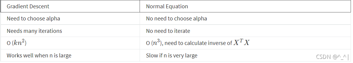
梯度下降法和正规方程法对比

在这里插入图片描述

matlab下演练

假设有数据特征矩阵X为47 $\times$ 2表示47个样本，2个特征。同时y表示结果矩阵，大小为为47 $\times$ 1。 $\theta$ 初始化为47 $\times$ 1的全零向量。

首先，一般会为其增加全1列（即 $h(\theta) = w_0+x_1w_1+x_2w_2$ 一般为 $w_0$ 补充 $x_0$ 为1）
X = [ones(m, 1) X];
归一化
mu = mean(X);
sigma = std(X);
X_norm = (X - mu)./sigma;
计算损失函数
J = sum((X* theta - y).^2)/(2*m);
梯度下降
for iter = 1:num_iters：
　　 theta = theta - alpha * (X’((Xtheta) - y)) / m;

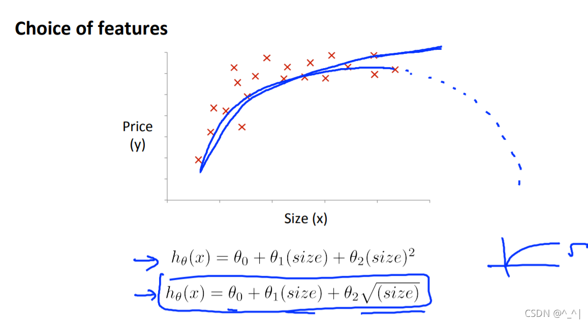
非线性化

在这里插入图片描述