机器学习数学基础之Python矩阵运算

Jupyter的七个基本实验

• 矩阵的加减行列转换：
  具体代码

import numpy as np
a = np.mat([[1, 2, 3], [4, 5, 6]])
a.shape
a.T
b = np.array([[1, 2, 3], [4, 5, 6]])
a + b
a - b

运行结果：

• 矩阵乘法

A = np.array([[1, 2, 3], [4, 5, 6]])
B = A.T
2 * A
np.dot(A, B)
np.dot( B, A)
C = np.array([[1, 2], [1, 3]])
np.dot(np.dot(A, B), C)
np.dot(A, np.dot(B, C))
A = B - 1
np.dot(A+B, C)
np.dot(A, C) + np.dot(B, C)
2*(np.dot(A, C))
np.dot(2*A, C)
np.dot(A, 2*C)
D = np.eye(2)
np.dot(C, D)

实现结果如下：

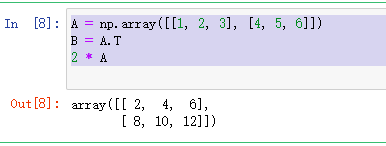
• 矩阵的数乘

A = np.array([[1, 2, 3], [4, 5, 6]])
B = A.T
2 * A

实现结果如下：

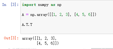
• 矩阵转置：

import numpy as np

A = np.array([[1, 2, 3], [4, 5, 6]])

A.T.T

运行结果：

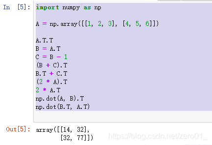
转置后求和：

import numpy as np

A = np.array([[1, 2, 3], [4, 5, 6]])

A.T.T
B = A.T
C = B - 1
(B + C).T
B.T + C.T
(2 * A).T
2 * A.T
np.dot(A, B).T
np.dot(B.T, A.T)

运行结果：

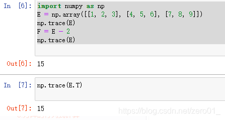
• 求矩阵的迹，验证方阵的迹等于方阵的转置的迹：

import numpy as np
E = np.array([[1, 2, 3], [4, 5, 6], [7, 8, 9]])
np.trace(E)
F = E - 2
np.trace(E)

运行结果：

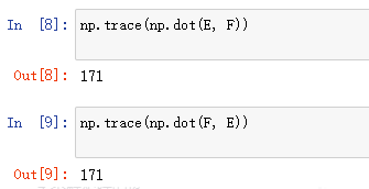
• 方阵乘积的迹：

np.trace(np.dot(E, F))
np.trace(np.dot(F, E))

运行结果：

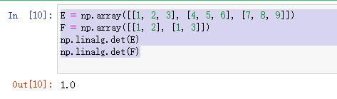
• 方针的行列式计算：

E = np.array([[1, 2, 3], [4, 5, 6], [7, 8, 9]])
F = np.array([[1, 2], [1, 3]])
np.linalg.det(E)
np.linalg.det(F)

运行结果：

• 矩阵的逆矩阵/伴随矩阵：

A = np.array([[1, -2, 1], [0, 2, -1], [1, 1, -2]])
B = np.linalg.inv(A)
A_abs = np.linalg.det(A)
B = np.linalg.inv(A)
A_bansui = B * A_abs

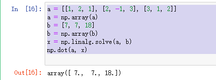
• 求解多元一次方程：

a = [[1, 2, 1], [2, -1, 3], [3, 1, 2]]
a = np.array(a)
b = [7, 7, 18]
b = np.array(b)
x = np.linalg.solve(a, b)
np.dot(a, x)

运行结果：

梯度下降法

微分

微分在数学中的定义：由函数B=f(A)，得到A、B两个数集，在A中当dx靠近自己时，函数在dx处的极限叫作函数在dx处的微分，微分的中心思想是无穷分割。微分是函数改变量的线性主要部分。微积分的基本概念之一

梯度

梯度的本意是一个向量（矢量），表示某一函数在该点处的方向导数沿着该方向取得最大值，即函数在该点处沿着该方向（此梯度的方向）变化最快，变化率最大（为该梯度的模）。

梯度下降法

在机器学习算法中，对于很多监督学习模型，需要对原始的模型构建损失函数，接下来便是通过优化算法对损失函数进行优化，以便寻找到最优的参数。在求解机器学习参数的优化算法中，使用较多的是基于梯度下降的优化算法(Gradient Descent, GD)。
梯度下降法有很多优点，其中，在梯度下降法的求解过程中，只需求解损失函数的一阶导数，计算的代价比较小，这使得梯度下降法能在很多大规模数据集上得到应用。梯度下降法的含义是通过当前点的梯度方向寻找到新的迭代点。

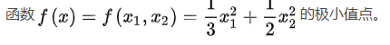
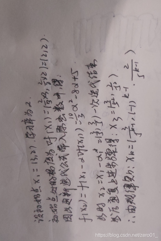
• 用梯度下降法手工求解
  

Excel利用梯度下降法求解近似根

• 初始设定：
  
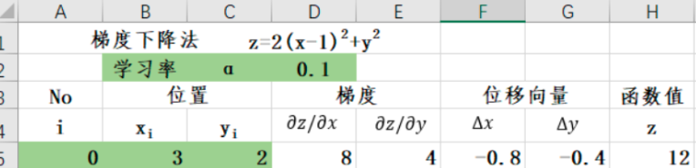
• 计算位移量：
  
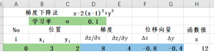
• 更新位置：
  
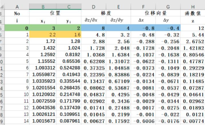
  所以函数z 在 (1,0) 处取得最小值 0。

python编程实现求解

• 导入需要的库：

# 导入所需库
import numpy as np
import matplotlib.pyplot as plt
import matplotlib as mpl
import math
from mpl_toolkits.mplot3d import Axes3D
import warnings

• 定义相关函数：

# 原函数
def Z(x,y):
    return 2*(x-1)**2 + y**2
# x方向上的梯度
def dx(x):
    return 4*x-4
# y方向上的梯度
def dy(y):
    return 2*y

• 重复迭代：

# 初始值
X = x_0 = 3
Y = y_0 = 2
# 学习率
alpha = 0.1
# 保存梯度下降所经过的点
globalX = [x_0]
globalY = [y_0]
globalZ = [Z(x_0,y_0)]
# 迭代30次
for i in range(30):
    temX = X - alpha * dx(X)
    temY = Y - alpha * dy(Y)
    temZ = Z(temX, temY)
    # X,Y 重新赋值
    X = temX
    Y = temY
    # 将新值存储起来
    globalX.append(temX)
    globalY.append(temY)
    globalZ.append(temZ)

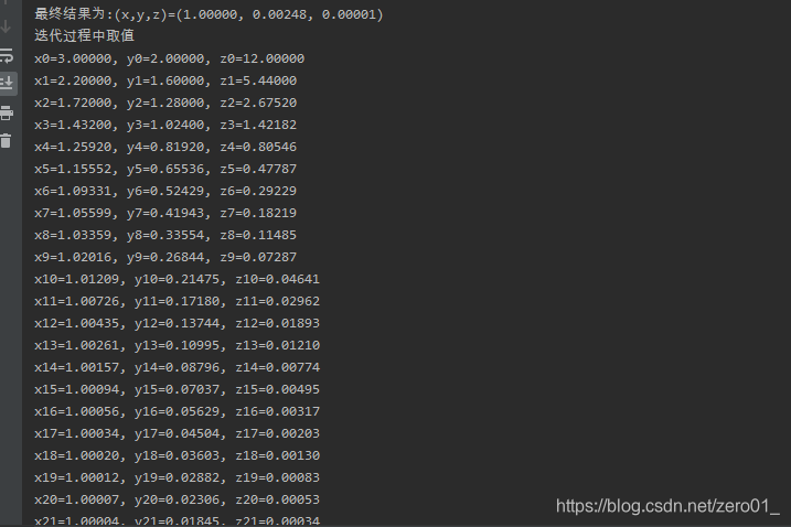
• 打印结果：

# 打印结果
print(u"最终结果为:(x,y,z)=(%.5f, %.5f, %.5f)" % (X, Y, Z(X,Y)))
print(u"迭代过程中取值")
num = len(globalX)
for i in range(num):
    print(u"x%d=%.5f, y%d=%.5f, z%d=%.5f" % (i,globalX[i],i,globalY[i],i,globalZ[i]))

运行结果：

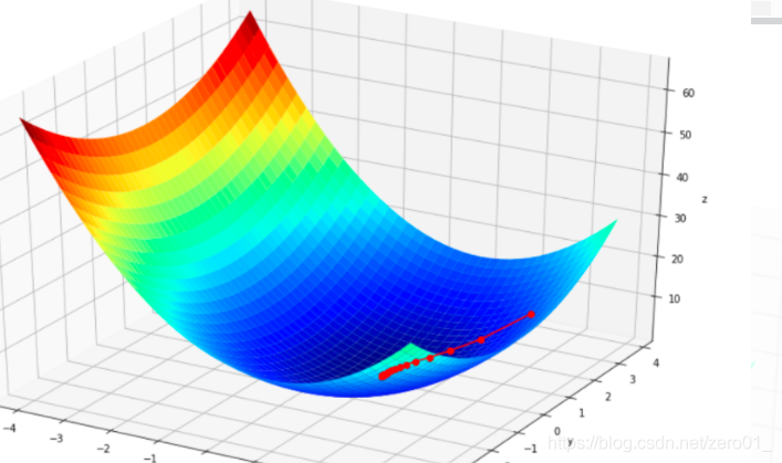
• 绘制过程;

%matplotlib inline
axisX = np.arange(-4,4,0.2)
axisY = np.arange(-4,4,0.2)
axisX, axisY = np.meshgrid(axisX, axisY) # 生成xv、yv，将axisX、axisY变成n*m的矩阵，方便后面绘图
valueZ = np.array(list(map(lambda t : Z(t[0],t[1]),zip(axisX.flatten(),axisY.flatten()))))
valueZ.shape = axisX.shape # 1600的Z图还原成原来的（40,40）
%matplotlib inline

#作图
fig = plt.figure(facecolor='w',figsize=(12,8))
ax = Axes3D(fig)
ax.plot_surface(axisX,axisY,valueZ,rstride=1,cstride=1,cmap=plt.cm.jet)
ax.plot(globalX,globalY,globalZ,'ko-')
ax.set_title(u'$ z=2×(x-1)^2 + y^2  $')
ax.set_xlabel(u'x')
ax.set_ylabel(u'y')
ax.set_zlabel('z')
plt.show()

运行结果：