kNN算法的快速使用及其代码实现（sklearn鸢尾花数据集实战）

在进行代码的书写之前，我们先讲述一下我们要使用的关键库sklearn，sklearn库里面有许多关键的包，对于他，后面会单独进行介绍，我们首先需要导入sklearn里面的datasets包，用于获取里面的鸢尾花数据集，以及sklearn里面的neighbors包 用于获取 KNeighborsClassifier模型。

我们还用到了一个很关键的数据分离操作模块：

train_test_split

它的一般形式为：

X_train,X_test, y_train, y_test = train_test_split(train_data, train_target, test_size, random_state, shuffle)

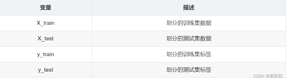
当然X_train这些都只是定义的变量名字而已，这些都可以自己去自定义的，这里就是想让大家知道它们对应的位置所对应的获取。

第一获取数据集

from sklearn import  datasets #导入数据集
from sklearn.neighbors import KNeighborsClassifier as KNN #导入KNN模型
from sklearn.model_selection import train_test_split #导入数据分离包 用法：X_train,X_test, y_train, y_test = train_test_split(train_data, train_target, test_size, random_state, shuffle)
import  numpy
data=datasets.load_iris()
#print(data)
key=data.keys()
#print(key) #dict_keys(['data', 'target', 'frame', 'target_names', 'DESCR', 'feature_names', 'filename', 'data_module'])
sample=data['data']
#print(sample)
#print(sample.shape)#(150, 4) 一共150行 每行数据都有四个特征
# print(data['target'])
# [0 0 0 0 0 0 0 0 0 0 0 0 0 0 0 0 0 0 0 0 0 0 0 0 0 0 0 0 0 0 0 0 0 0 0 0 0
#  0 0 0 0 0 0 0 0 0 0 0 0 0 1 1 1 1 1 1 1 1 1 1 1 1 1 1 1 1 1 1 1 1 1 1 1 1
#  1 1 1 1 1 1 1 1 1 1 1 1 1 1 1 1 1 1 1 1 1 1 1 1 1 1 2 2 2 2 2 2 2 2 2 2 2
#  2 2 2 2 2 2 2 2 2 2 2 2 2 2 2 2 2 2 2 2 2 2 2 2 2 2 2 2 2 2 2 2 2 2 2 2 2
#  2 2]
target=data['target']
#print(data['target_names'])#['setosa' 'versicolor' 'virginica']三种类型分别对应：0，1，2
b={0:'setosa',1:'versicolor',2:'virginica'}#简单构造一个类型和标签对应的字典，为了后面使用的方便

上面的大家应该都能看明白吧，定义了一个data变量用于获取鸢尾花数据集，将其输出的话是这样的：

D:\Anaconda3\python.exe D:\pythonProject\机器学习\KNN模型使用.py 
{'data': array([[5.1, 3.5, 1.4, 0.2],
       [4.9, 3. , 1.4, 0.2],
       [4.7, 3.2, 1.3, 0.2],
       [4.6, 3.1, 1.5, 0.2],
       [5. , 3.6, 1.4, 0.2],
       [5.4, 3.9, 1.7, 0.4],
       [4.6, 3.4, 1.4, 0.3],
       [5. , 3.4, 1.5, 0.2],
       [4.4, 2.9, 1.4, 0.2],
       [4.9, 3.1, 1.5, 0.1],
       [5.4, 3.7, 1.5, 0.2],
       [4.8, 3.4, 1.6, 0.2],
       [4.8, 3. , 1.4, 0.1],
       [4.3, 3. , 1.1, 0.1],
       [5.8, 4. , 1.2, 0.2],
       [5.7, 4.4, 1.5, 0.4],
       [5.4, 3.9, 1.3, 0.4],
       [5.1, 3.5, 1.4, 0.3],
       [5.7, 3.8, 1.7, 0.3],
       [5.1, 3.8, 1.5, 0.3],
       [5.4, 3.4, 1.7, 0.2],
       [5.1, 3.7, 1.5, 0.4],
       [4.6, 3.6, 1. , 0.2],
       [5.1, 3.3, 1.7, 0.5],
       [4.8, 3.4, 1.9, 0.2],
       [5. , 3. , 1.6, 0.2],
       [5. , 3.4, 1.6, 0.4],
       [5.2, 3.5, 1.5, 0.2],
       [5.2, 3.4, 1.4, 0.2],
       [4.7, 3.2, 1.6, 0.2],
       [4.8, 3.1, 1.6, 0.2],
       [5.4, 3.4, 1.5, 0.4],
       [5.2, 4.1, 1.5, 0.1],
       [5.5, 4.2, 1.4, 0.2],
       [4.9, 3.1, 1.5, 0.2],
       [5. , 3.2, 1.2, 0.2],
       [5.5, 3.5, 1.3, 0.2],
       [4.9, 3.6, 1.4, 0.1],
       [4.4, 3. , 1.3, 0.2],
       [5.1, 3.4, 1.5, 0.2],
       [5. , 3.5, 1.3, 0.3],
       [4.5, 2.3, 1.3, 0.3],
       [4.4, 3.2, 1.3, 0.2],
       [5. , 3.5, 1.6, 0.6],
       [5.1, 3.8, 1.9, 0.4],
       [4.8, 3. , 1.4, 0.3],
       [5.1, 3.8, 1.6, 0.2],
       [4.6, 3.2, 1.4, 0.2],
       [5.3, 3.7, 1.5, 0.2],
       [5. , 3.3, 1.4, 0.2],
       [7. , 3.2, 4.7, 1.4],
       [6.4, 3.2, 4.5, 1.5],
       [6.9, 3.1, 4.9, 1.5],
       [5.5, 2.3, 4. , 1.3],
       [6.5, 2.8, 4.6, 1.5],
       [5.7, 2.8, 4.5, 1.3],
       [6.3, 3.3, 4.7, 1.6],
       [4.9, 2.4, 3.3, 1. ],
       [6.6, 2.9, 4.6, 1.3],
       [5.2, 2.7, 3.9, 1.4],
       [5. , 2. , 3.5, 1. ],
       [5.9, 3. , 4.2, 1.5],
       [6. , 2.2, 4. , 1. ],
       [6.1, 2.9, 4.7, 1.4],
       [5.6, 2.9, 3.6, 1.3],
       [6.7, 3.1, 4.4, 1.4],
       [5.6, 3. , 4.5, 1.5],
       [5.8, 2.7, 4.1, 1. ],
       [6.2, 2.2, 4.5, 1.5],
       [5.6, 2.5, 3.9, 1.1],
       [5.9, 3.2, 4.8, 1.8],
       [6.1, 2.8, 4. , 1.3],
       [6.3, 2.5, 4.9, 1.5],
       [6.1, 2.8, 4.7, 1.2],
       [6.4, 2.9, 4.3, 1.3],
       [6.6, 3. , 4.4, 1.4],
       [6.8, 2.8, 4.8, 1.4],
       [6.7, 3. , 5. , 1.7],
       [6. , 2.9, 4.5, 1.5],
       [5.7, 2.6, 3.5, 1. ],
       [5.5, 2.4, 3.8, 1.1],
       [5.5, 2.4, 3.7, 1. ],
       [5.8, 2.7, 3.9, 1.2],
       [6. , 2.7, 5.1, 1.6],
       [5.4, 3. , 4.5, 1.5],
       [6. , 3.4, 4.5, 1.6],
       [6.7, 3.1, 4.7, 1.5],
       [6.3, 2.3, 4.4, 1.3],
       [5.6, 3. , 4.1, 1.3],
       [5.5, 2.5, 4. , 1.3],
       [5.5, 2.6, 4.4, 1.2],
       [6.1, 3. , 4.6, 1.4],
       [5.8, 2.6, 4. , 1.2],
       [5. , 2.3, 3.3, 1. ],
       [5.6, 2.7, 4.2, 1.3],
       [5.7, 3. , 4.2, 1.2],
       [5.7, 2.9, 4.2, 1.3],
       [6.2, 2.9, 4.3, 1.3],
       [5.1, 2.5, 3. , 1.1],
       [5.7, 2.8, 4.1, 1.3],
       [6.3, 3.3, 6. , 2.5],
       [5.8, 2.7, 5.1, 1.9],
       [7.1, 3. , 5.9, 2.1],
       [6.3, 2.9, 5.6, 1.8],
       [6.5, 3. , 5.8, 2.2],
       [7.6, 3. , 6.6, 2.1],
       [4.9, 2.5, 4.5, 1.7],
       [7.3, 2.9, 6.3, 1.8],
       [6.7, 2.5, 5.8, 1.8],
       [7.2, 3.6, 6.1, 2.5],
       [6.5, 3.2, 5.1, 2. ],
       [6.4, 2.7, 5.3, 1.9],
       [6.8, 3. , 5.5, 2.1],
       [5.7, 2.5, 5. , 2. ],
       [5.8, 2.8, 5.1, 2.4],
       [6.4, 3.2, 5.3, 2.3],
       [6.5, 3. , 5.5, 1.8],
       [7.7, 3.8, 6.7, 2.2],
       [7.7, 2.6, 6.9, 2.3],
       [6. , 2.2, 5. , 1.5],
       [6.9, 3.2, 5.7, 2.3],
       [5.6, 2.8, 4.9, 2. ],
       [7.7, 2.8, 6.7, 2. ],
       [6.3, 2.7, 4.9, 1.8],
       [6.7, 3.3, 5.7, 2.1],
       [7.2, 3.2, 6. , 1.8],
       [6.2, 2.8, 4.8, 1.8],
       [6.1, 3. , 4.9, 1.8],
       [6.4, 2.8, 5.6, 2.1],
       [7.2, 3. , 5.8, 1.6],
       [7.4, 2.8, 6.1, 1.9],
       [7.9, 3.8, 6.4, 2. ],
       [6.4, 2.8, 5.6, 2.2],
       [6.3, 2.8, 5.1, 1.5],
       [6.1, 2.6, 5.6, 1.4],
       [7.7, 3. , 6.1, 2.3],
       [6.3, 3.4, 5.6, 2.4],
       [6.4, 3.1, 5.5, 1.8],
       [6. , 3. , 4.8, 1.8],
       [6.9, 3.1, 5.4, 2.1],
       [6.7, 3.1, 5.6, 2.4],
       [6.9, 3.1, 5.1, 2.3],
       [5.8, 2.7, 5.1, 1.9],
       [6.8, 3.2, 5.9, 2.3],
       [6.7, 3.3, 5.7, 2.5],
       [6.7, 3. , 5.2, 2.3],
       [6.3, 2.5, 5. , 1.9],
       [6.5, 3. , 5.2, 2. ],
       [6.2, 3.4, 5.4, 2.3],
       [5.9, 3. , 5.1, 1.8]]), 'target': array([0, 0, 0, 0, 0, 0, 0, 0, 0, 0, 0, 0, 0, 0, 0, 0, 0, 0, 0, 0, 0, 0,
       0, 0, 0, 0, 0, 0, 0, 0, 0, 0, 0, 0, 0, 0, 0, 0, 0, 0, 0, 0, 0, 0,
       0, 0, 0, 0, 0, 0, 1, 1, 1, 1, 1, 1, 1, 1, 1, 1, 1, 1, 1, 1, 1, 1,
       1, 1, 1, 1, 1, 1, 1, 1, 1, 1, 1, 1, 1, 1, 1, 1, 1, 1, 1, 1, 1, 1,
       1, 1, 1, 1, 1, 1, 1, 1, 1, 1, 1, 1, 2, 2, 2, 2, 2, 2, 2, 2, 2, 2,
       2, 2, 2, 2, 2, 2, 2, 2, 2, 2, 2, 2, 2, 2, 2, 2, 2, 2, 2, 2, 2, 2,
       2, 2, 2, 2, 2, 2, 2, 2, 2, 2, 2, 2, 2, 2, 2, 2, 2, 2]), 'frame': None, 'target_names': array(['setosa', 'versicolor', 'virginica'], dtype='<U10'), 'DESCR': '.. _iris_dataset:\n\nIris plants dataset\n--------------------\n\n**Data Set Characteristics:**\n\n    :Number of Instances: 150 (50 in each of three classes)\n    :Number of Attributes: 4 numeric, predictive attributes and the class\n    :Attribute Information:\n        - sepal length in cm\n        - sepal width in cm\n        - petal length in cm\n        - petal width in cm\n        - class:\n                - Iris-Setosa\n                - Iris-Versicolour\n                - Iris-Virginica\n                \n    :Summary Statistics:\n\n    ============== ==== ==== ======= ===== ====================\n                    Min  Max   Mean    SD   Class Correlation\n    ============== ==== ==== ======= ===== ====================\n    sepal length:   4.3  7.9   5.84   0.83    0.7826\n    sepal width:    2.0  4.4   3.05   0.43   -0.4194\n    petal length:   1.0  6.9   3.76   1.76    0.9490  (high!)\n    petal width:    0.1  2.5   1.20   0.76    0.9565  (high!)\n    ============== ==== ==== ======= ===== ====================\n\n    :Missing Attribute Values: None\n    :Class Distribution: 33.3% for each of 3 classes.\n    :Creator: R.A. Fisher\n    :Donor: Michael Marshall (MARSHALL%PLU@io.arc.nasa.gov)\n    :Date: July, 1988\n\nThe famous Iris database, first used by Sir R.A. Fisher. The dataset is taken\nfrom Fisher\'s paper. Note that it\'s the same as in R, but not as in the UCI\nMachine Learning Repository, which has two wrong data points.\n\nThis is perhaps the best known database to be found in the\npattern recognition literature.  Fisher\'s paper is a classic in the field and\nis referenced frequently to this day.  (See Duda & Hart, for example.)  The\ndata set contains 3 classes of 50 instances each, where each class refers to a\ntype of iris plant.  One class is linearly separable from the other 2; the\nlatter are NOT linearly separable from each other.\n\n.. topic:: References\n\n   - Fisher, R.A. "The use of multiple measurements in taxonomic problems"\n     Annual Eugenics, 7, Part II, 179-188 (1936); also in "Contributions to\n     Mathematical Statistics" (John Wiley, NY, 1950).\n   - Duda, R.O., & Hart, P.E. (1973) Pattern Classification and Scene Analysis.\n     (Q327.D83) John Wiley & Sons.  ISBN 0-471-22361-1.  See page 218.\n   - Dasarathy, B.V. (1980) "Nosing Around the Neighborhood: A New System\n     Structure and Classification Rule for Recognition in Partially Exposed\n     Environments".  IEEE Transactions on Pattern Analysis and Machine\n     Intelligence, Vol. PAMI-2, No. 1, 67-71.\n   - Gates, G.W. (1972) "The Reduced Nearest Neighbor Rule".  IEEE Transactions\n     on Information Theory, May 1972, 431-433.\n   - See also: 1988 MLC Proceedings, 54-64.  Cheeseman et al"s AUTOCLASS II\n     conceptual clustering system finds 3 classes in the data.\n   - Many, many more ...', 'feature_names': ['sepal length (cm)', 'sepal width (cm)', 'petal length (cm)', 'petal width (cm)'], 'filename': 'iris.csv', 'data_module': 'sklearn.datasets.data'}

进程已结束,退出代码0

而我们用变量sample接受了所有的特征样本数据，也就是数据集里面‘data’对应的数据。至于我们定义的target得到的是什么注释上已经很清楚了。

第二对数据集进行处理，得到测试数据集和训练数据集

#数据分离
traindata,testdata,traintarget,testtarget = train_test_split(sample,target,test_size=0.1,random_state=2020)
print(traindata.shape)#(135, 4)
print(testdata.shape)#(15, 4)

上面已经介绍过train_test_split（）返回值是什么还有怎么用了，所以这里就不看traindata这四个输出的内容了，下面是我们设定的训练集和测试集的shape因为我们在train_test_split里面的test_size（这个顾名思义就是测试集占比）设置的是0.1，所以测试集就占总数据集的十分之一。

第三：使用模型KNeighborsClassifier用于knn算法的实现，并自定k的值

#调用KNN模型
knn=KNN(n_neighbors=4) #k值设为4
knn.fit(traindata,traintarget)#使用训练集数据训练模型  traindata:训练集的特征数据,特征数据的维度必须是二维     traintarget:训练集的标签数据,一维的

第四训练模型，得到准确度

pred=knn.predict(testdata) #利用训练的模型预测结果
print('测数据集预测的结果:',pred)
print('真实的结果:',testtarget)
print(knn.score(traindata,traintarget))#预测训练集的结果与训练集真实结果相比的准确度

第五预测

#预测数据
a=[[14,20,20,45]]
a=numpy.array(a)
print(knn.predict(a))
print(b[knn.predict(a)[0]])

以上所有过程的完整源代码

from sklearn import  datasets #导入数据集
from sklearn.neighbors import KNeighborsClassifier as KNN #导入KNN模型
from sklearn.model_selection import train_test_split #导入数据分离包 用法：X_train,X_test, y_train, y_test = train_test_split(train_data, train_target, test_size, random_state, shuffle)
import  numpy
data=datasets.load_iris()
#print(data)
key=data.keys()
#print(key) #dict_keys(['data', 'target', 'frame', 'target_names', 'DESCR', 'feature_names', 'filename', 'data_module'])
sample=data['data']
#print(sample)
#print(sample.shape)#(150, 4) 一共150行 每行数据都有四个特征
# print(data['target'])
# [0 0 0 0 0 0 0 0 0 0 0 0 0 0 0 0 0 0 0 0 0 0 0 0 0 0 0 0 0 0 0 0 0 0 0 0 0
#  0 0 0 0 0 0 0 0 0 0 0 0 0 1 1 1 1 1 1 1 1 1 1 1 1 1 1 1 1 1 1 1 1 1 1 1 1
#  1 1 1 1 1 1 1 1 1 1 1 1 1 1 1 1 1 1 1 1 1 1 1 1 1 1 2 2 2 2 2 2 2 2 2 2 2
#  2 2 2 2 2 2 2 2 2 2 2 2 2 2 2 2 2 2 2 2 2 2 2 2 2 2 2 2 2 2 2 2 2 2 2 2 2
#  2 2]
target=data['target']
#print(data['target_names'])#['setosa' 'versicolor' 'virginica']三种类型分别对应：0，1，2
b={0:'setosa',1:'versicolor',2:'virginica'}#简单构造一个类型和标签对应的字典，为了后面使用的方便
#数据分离
traindata,testdata,traintarget,testtarget = train_test_split(sample,target,test_size=0.1,random_state=2020)
print(traindata.shape)#(135, 4)
print(testdata.shape)#(15, 4)
#调用KNN模型
knn=KNN(n_neighbors=4) #k值设为4
knn.fit(traindata,traintarget)#使用训练集数据训练模型  traindata:训练集的特征数据,特征数据的维度必须是二维     traintarget:训练集的标签数据,一维的
pred=knn.predict(testdata) #利用训练的模型预测结果
print('测数据集预测的结果:',pred)
print('真实的结果:',testtarget)
print(knn.score(traindata,traintarget))#预测训练集的结果与训练集真实结果相比的准确度
#预测数据
a=[[14,20,20,45]]
a=numpy.array(a)
print(knn.predict(a))
print(b[knn.predict(a)[0]])

第六模型的优化

对于该模型而言有两个优化模型的方向，第一就是k值的选择，第二就是测试集和训练集的选择

我们这里只讲述k值的优化，优化方法为K值交叉验证

K值交叉验证是什么意思呢？

将样本的训练数据交叉的拆分出不同的训练集和验证集，使用交叉拆分出不同的训练集和验证集测分别试模型的精准度，然就求出的精准度的均值就是此次交叉验证的结果。将交叉验证作用到不同的超参数中，选取出精准度最高的超参数作为模型创建的超参数即可!

实现思路:

（1）将数据集平均分割成K个等份

（2）使用1份数据作为测试数据，其余作为训练数据

（3）计算测试准确率

（4）使用不同的测试集，重复2、3步骤

（5）对准确率做平均，作为对未知数据预测准确率的估计

实现：

首先我们要引入cross_val_score模块，这个功能模块在sklearn里面的model_selection包里面，为了显示方便我们会引入 matplotlib库里面的pyplot用于画图，更直观的显示。

下面是导入代码：

from sklearn.model_selection import cross_val_score
import  matplotlib.pyplot as plt

在此之前，我们有必要了解一下cross_val_score模块

cross_val_score参数设置
sklearn.model_selection.cross_val_score(estimator, X, y=None, groups=None, scoring=None, cv=’warn’, n_jobs=None, verbose=0, fit_params=None, pre_dispatch=‘2*n_jobs’, error_score=’raise-deprecating’)
参数：

estimator：需要使用交叉验证的算法应该说模型更恰当，我们在这里就直接写knn就好
X：输入样本数据
y：样本标签
groups：将数据集分割为训练/测试集时使用的样本的组标签（一般用不到）
scoring：交叉验证最重要的就是他的验证方式，选择不同的评价方法，会产生不同的评价结果

（下面的这张图片来源网络，侵权必删！）

cv：交叉验证折数或可迭代的次数
n_jobs：同时工作的cpu个数（-1代表全部）
verbose：详细程度
fit_params：传递给估计器（验证算法）的拟合方法的参数
pre_dispatch：控制并行执行期间调度的作业数量。减少这个数量对于避免在CPU发送更多作业时CPU内存消耗的扩大是有用的。该参数可以是：
一个int，给出所产生的总工作的确切数量
一个字符串，给出一个表达式作为n_jobs的函数，如’2 * n_jobs
error_score：如果在估计器拟合中发生错误，要分配给该分数的值（一般不需要指定）

以上便是关于cross_val_score参数设置的详细内容，看起来很多，其实我们至于要记住几个常用的就好，就像

estimator：
X
y

这四个，就是常用的，也是我们本次使用的，我们在本篇博客只需要记一下这四个参数的用法就好，cv我们本次设置为10也就是分为了10份，cross_val_score的返回值就是我们的模型在k值之下对应的准确度。

我们只需要在原来代码的基础上修改一下就好。

代码如下：

from sklearn import  datasets #导入数据集
from sklearn.neighbors import KNeighborsClassifier as KNN #导入KNN模型
from sklearn.model_selection import train_test_split #导入数据分离包 用法：X_train,X_test, y_train, y_test = train_test_split(train_data, train_target, test_size, random_state, shuffle)
import  numpy
from sklearn.model_selection import cross_val_score
import  matplotlib.pyplot as plt
data=datasets.load_iris()
#print(data)
key=data.keys()
#print(key) #dict_keys(['data', 'target', 'frame', 'target_names', 'DESCR', 'feature_names', 'filename', 'data_module'])
sample=data['data']
#print(sample)
#print(sample.shape)#(150, 4) 一共150行 每行数据都有四个特征
# print(data['target'])
# [0 0 0 0 0 0 0 0 0 0 0 0 0 0 0 0 0 0 0 0 0 0 0 0 0 0 0 0 0 0 0 0 0 0 0 0 0
#  0 0 0 0 0 0 0 0 0 0 0 0 0 1 1 1 1 1 1 1 1 1 1 1 1 1 1 1 1 1 1 1 1 1 1 1 1
#  1 1 1 1 1 1 1 1 1 1 1 1 1 1 1 1 1 1 1 1 1 1 1 1 1 1 2 2 2 2 2 2 2 2 2 2 2
#  2 2 2 2 2 2 2 2 2 2 2 2 2 2 2 2 2 2 2 2 2 2 2 2 2 2 2 2 2 2 2 2 2 2 2 2 2
#  2 2]
target=data['target']
#print(data['target_names'])#['setosa' 'versicolor' 'virginica']三种类型分别对应：0，1，2
b={0:'setosa',1:'versicolor',2:'virginica'}#简单构造一个类型和标签对应的字典，为了后面使用的方便
#数据分离
traindata,testdata,traintarget,testtarget = train_test_split(sample,target,test_size=0.1,random_state=2020)
print(traindata.shape)#(135, 4)
print(testdata.shape)#(15, 4)
#调用KNN模型
# knn=KNN(n_neighbors=4) #k值设为4
# knn.fit(traindata,traintarget)#使用训练集数据训练模型  traindata:训练集的特征数据,特征数据的维度必须是二维     traintarget:训练集的标签数据,一维的
# pred=knn.predict(testdata) #利用训练的模型预测结果
# print('测数据集预测的结果:',pred)
# print('真实的结果:',testtarget)
# print(knn.score(traindata,traintarget))#预测训练集的结果与训练集真实结果相比的准确度
# #预测数据
# a=[[14,20,20,45]]
# a=numpy.array(a)
# print(knn.predict(a))
# print(b[knn.predict(a)[0]])
pre=[]
k=[]
for i in range(3,20):
    knn=KNN(n_neighbors=i)
    pr=cross_val_score(knn,traindata,traintarget,cv=10).mean()#得到每次预测的平均值
    #print(pr)
    pre.append(pr)
    k.append(i)
# print(pre)
# print(k)
plt.plot(k,pre)
plt.show()

上面就是k值的选择和准确度的图像，总而言之我们使用的这个优化方法，它总归是一种优化方法，我们的目的是以此对准确率做平均，作为对未知数据预测准确率的估计。

这才是我们应当注意的。

注意

好了到此为止了，另外做个补充，在运行代码时候可能会出现这样的一个报错（D:\Anaconda3\lib\site-packages\sklearn\neighbors\_classification.py:228: FutureWarning: Unlike other reduction functions (e.g. `skew`, `kurtosis`), the default behavior of `mode` typically preserves the axis it acts along. In SciPy 1.11.0, this behavior will change: the default value of `keepdims` will become False, the `axis` over which the statistic is taken will be eliminated, and the value None will no longer be accepted. Set `keepdims` to True or False to avoid this warning.
mode, _ = stats.mode(_y[neigh_ind, k], axis=1)）

这个报错并不影响我们的代码的书写，以及结果的展示，也就是说我们不用管他，这个报错感兴趣可以查一下，我这里就不解释了，只是一个可以忽略的小问题。