


单目稠密重建
极线搜索与块匹配
如图所示,左边的相机观测到了某个像素p1,由于这是一个单目相机,我们无从知道它的深度。
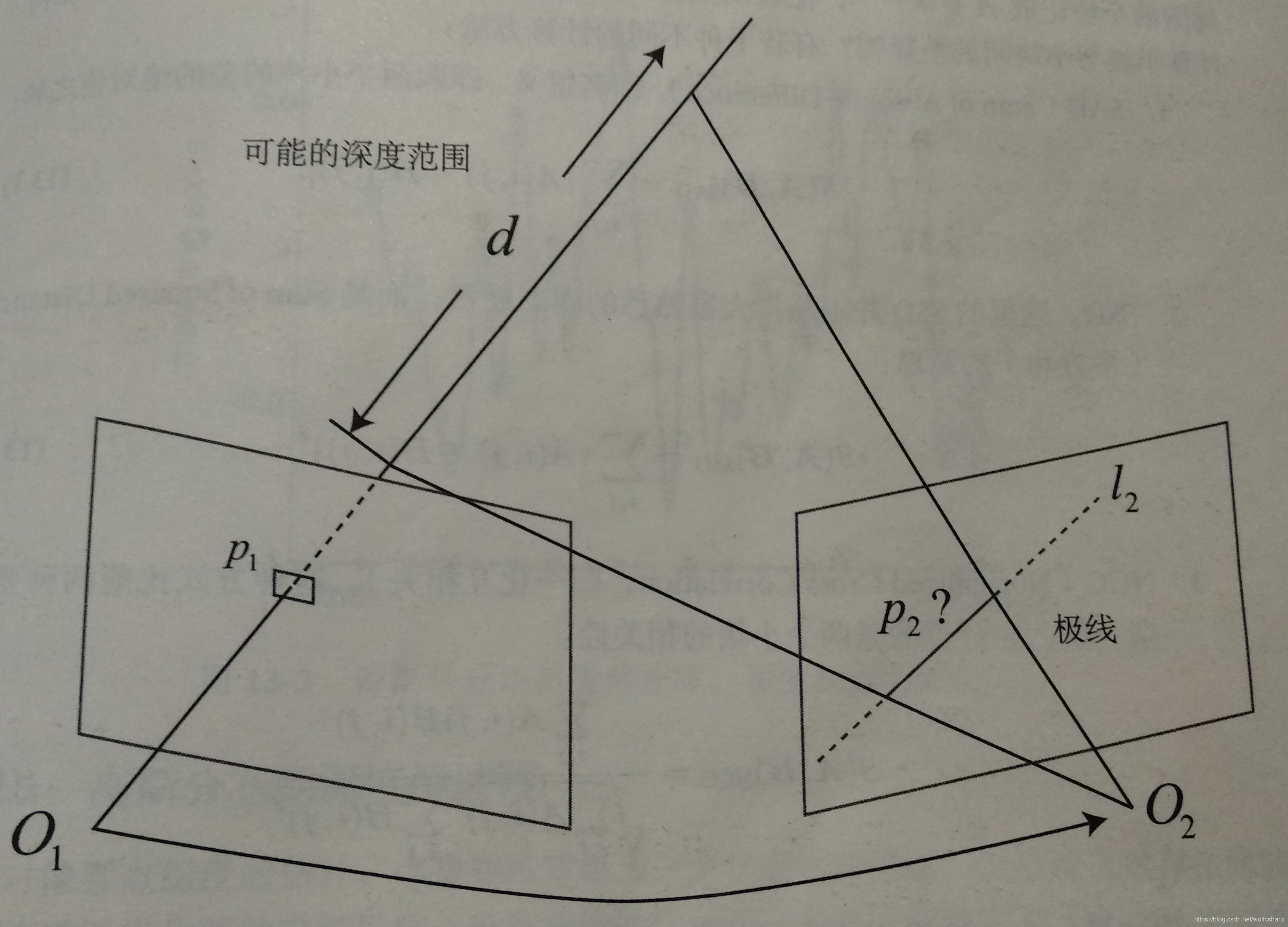
就像对极几何中描述的一样,p1对应的空间点会落在右边相机拍摄的图像的极线l2上。
在特征点方法中,极线基本没有意义,因为我们通过特征匹配直接可以找到p2的位置。但是现在我们要建立稠密地图,没有描述子,所以只能在极线上搜索和p1长的比较相似的点。
单个像素灰度值含有的信息量较小,比较单个像素的灰度没有区分性,因此我们考虑在p1周围取一个大小为w×w的小块,然后在极线上也取很多同样大小的小块进行比较,就可以在一定程度上提高区分性,这就是块匹配。
块相似性的衡量方法:
把p1周围的小块记成A(属于Rw×w),把极线上的n个小块记成Bi,i=1,…,n,有如下若干种不同的相似性计算方法:
-
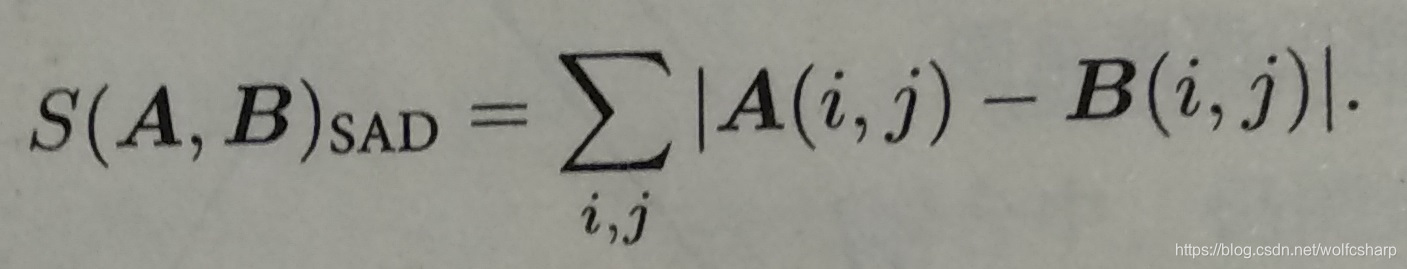
SAD(Sum of Absolute Difference):
-
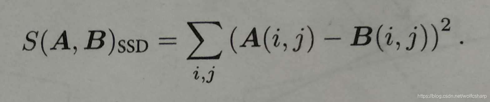
SSD(Sum of Squared Distance):
-
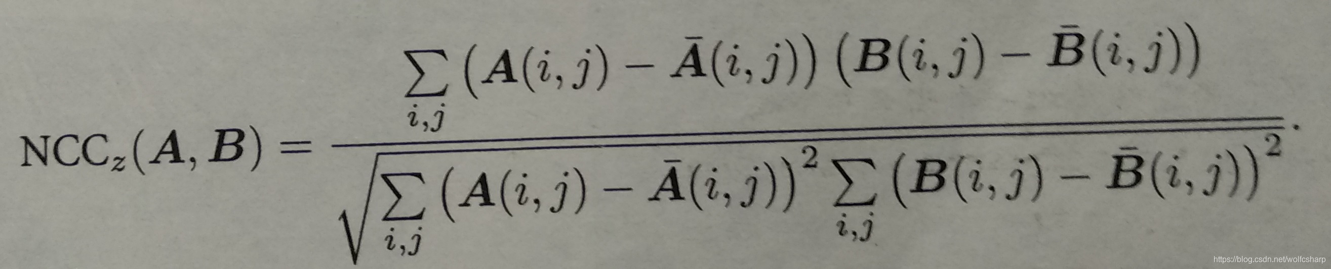
NCC(Normalized Cross Correlation,归一化互相关):
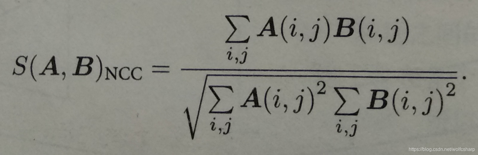
注意:SAD和SSD是数值越小(接近0)相似性越大,数值越大相似性越小;NCC则是表示相关性,数值接近1表示两幅图像相似,而数值接近0表示两幅图像不相似。
NCC方法的极线搜索和块匹配得分图: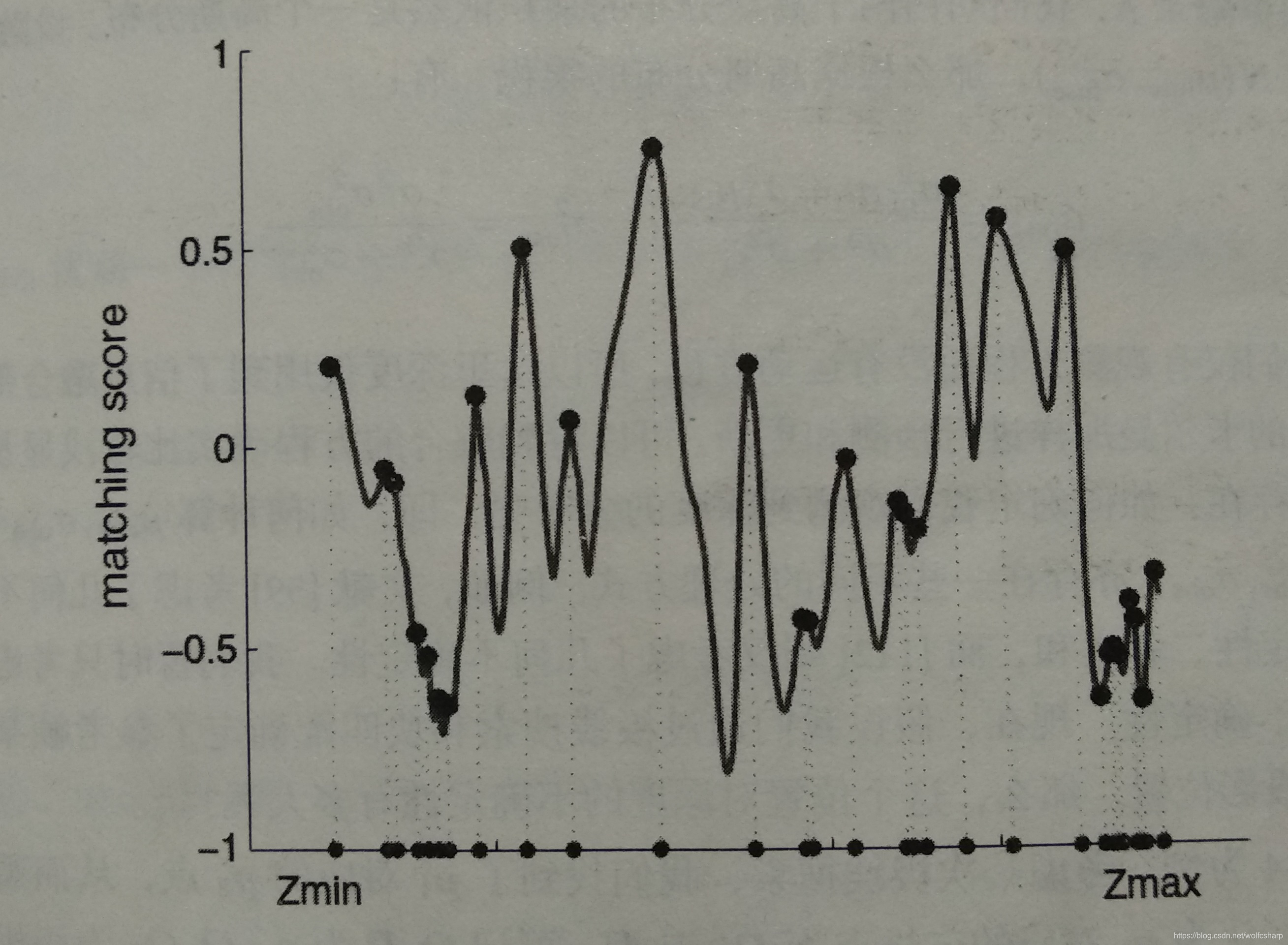
在搜索距离较长的情况下,我们通常会得到一个非凸函数:这个分布存在着许多峰值,然而真实的对应点p2必定只有一个。在这种情况下,我们会倾向于使用概率分布来描述深度值,而非采用某个单一的数值来描述深度。
高斯分布的深度滤波器
设某个像素点p1的深度d服从:
以第一幅图作为参考,后续的图像观测将对第一幅图的深度d进行更新。
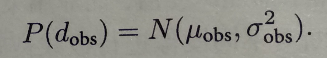
而每当新的数据到来,我们都会观测到它的深度。同样,假设这次观测也是一个高斯分布:
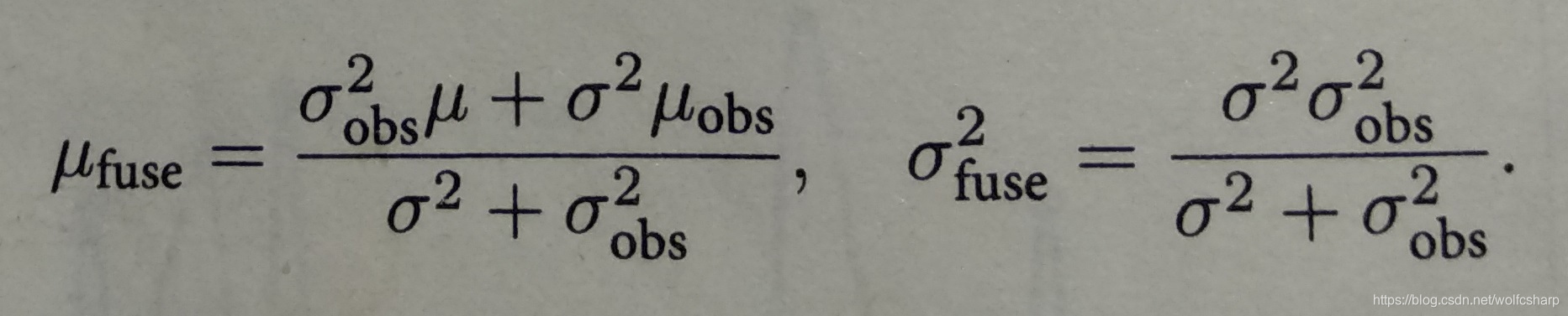
为了使用观测的信息更新原来d的分布,我们需要对高斯分布进行信息融合,融合之后d的分布为:
观测d的分布的处理:
只考虑几何不确定性,假设我们通过极线搜索和块匹配确定了参考帧某个像素在当前帧的投影位置。那么,这个位置对深度的不确定性有多大呢?
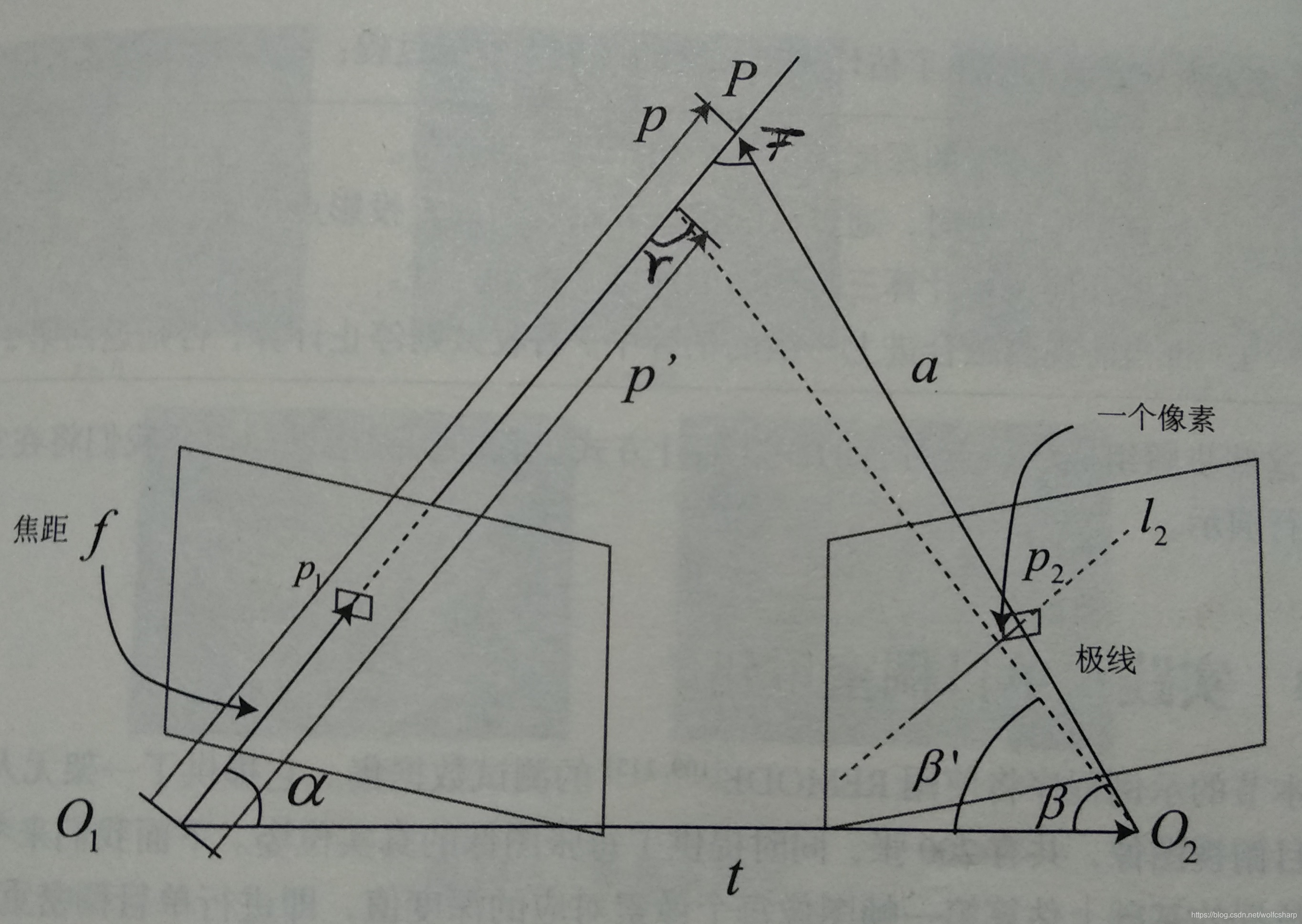
以上图为例,考虑某次极线搜索,我们找到了p1对应的p2点,从而观测到了p1的深度值,认为p1对应的三维点为P。从而,可记O1P为p,O1O2为相机的平移t,O2P记为a.并且,把这个三角形的下面两个角记作alpha,beta。
现在,考虑极线l2上存在着一个像素大小的误差,使得beta角变成了beta‘,而p也变成了p’,并记上面那个角为gamma。我们要问的是,这一个像素的误差会导致p’与p产生多大的差距呢?
这是一个典型的几何问题。我们来列写这些量之间的几何关系。显然有:
a = p - t
alpha = arccos(p,t)
beta = arccos(a,-t)
对p2扰动一个像素,将使得beta产生一个变化量delta_beta,由于相机焦距为f,于是:
delta_beta = arctan(1/f)
所以:
beta’ = beta + delta_beta
gamma = pi - alpha - beta’
于是,根据正弦定理,p’的大小可以求得:
||p’|| = ||t||sin(bata’)/sin(gamma)
由此,我们确定了单个像素的不确定引起的深度不确定性。如果认为极线搜索的块匹配仅有一个像素的误差,那么就可以设:

综上所述,我们给出了估计稠密深度的一个完整过程:
- 假设所有像素的深度满足某个初始的高斯分布
- 当新数据产生时,通过极线搜索和块匹配确定投影点位置
- 根据几何关系计算三角化后的深度及不确定性
- 将当前观测融合进上一次的估计中。若收敛则停止计算,否则返回第2步。
实践:单目稠密重建
关键函数的说明:
1.main函数负责从数据集中读取图像,然后交给update函数,对深度图进行更新。
2.update函数遍历了参考帧的每个像素,先在当前帧中寻找极线匹配,若能匹配上,则利用极线匹配的结果更新深度图的估计。
3.极线搜索的实现:假设深度值服从高斯分布,我们以均值为中心,左右各取±3sigma作为半径,然后在当前帧中寻找极线的投影。再遍历此极线上的像素(步长取sqrt(2)/2的近似值0.7),寻找NCC最高的点作为匹配点。如果最高的NCC也低于阈值(这里取0.85),则认为匹配失败。
4.NCC的计算使用了取均值化后的做法,即对于图像块A,B,取:
5.三角化代码解析参看代码
6.不确定性的计算与高斯融合方法和上一节一致
完整代码
dense_monocular/dense_mapping.cpp
//2019.08.18
#include <iostream>
#include <vector>
#include <fstream>
using namespace std;
#include <boost/timer.hpp>

//for sophus
#include <sophus/se3.h>
using Sophus::SE3;

//for Eigen
#include <Eigen/Core>
#include <Eigen/Geometry>
using namespace Eigen;

//for opencv
#include <opencv2/core/core.hpp>
#include <opencv2/highgui/highgui.hpp>
#include <opencv2/imgproc/imgproc.hpp>
using namespace cv;


/**********************************
*本程序演示了单目相机在已知轨迹下的稠密深度估计
*使用极线搜索中 + NCC匹配的方式
*程序仍然有改进的空间
***********************************/

//parameters
const int border = 20;//边缘宽度
const int width = 640;//宽度
const int height = 480;//高度f
const double fx = 481.2f;//相机内参
const double fy = -480.0f;
const double cx = 319.5f;
const double cy = 239.5f;
const int ncc_window_size = 2;//NCC取的窗口半宽度
const int ncc_area = (2*ncc_window_size+1)*(2*ncc_window_size+1);//NCC窗口面积
const double min_cov = 0.1;//收敛判定:最小方差
const double max_cov = 10;//收敛判定:最大方差


//-------------------------------------------------------------------------------------------------
//一些小工具

//1.显示估计的深度图
bool plotDepth(const Mat& depth)
{
	imshow( "depth", depth*0.4 );
	waitKey(1);
}

//2.像素到相机坐标系的转换
inline Vector3d px2cam(const Vector2d px)
{
	return Vector3d((px(0,0) - cx)/fx, (px(1,0) - cy)/fy, 1 );
}


//3.相机坐标到像素坐标的转换
inline Vector2d cam2px(const Vector3d p_cam)
{
	return Vector2d(p_cam(0,0)*fx/p_cam(2,0) + cx, p_cam(1,0)*fy/p_cam(2,0) + cy);
}


//4.检测一个点是否在图像边框内
inline bool inside(const Vector2d& pt)
{
	return pt(0,0)>=border && pt(1,0)>=border && pt(0,0)+border<width && pt(1,0)+border<=height;
}


//5.显示极线匹配
void showEpipolarMatch(const Mat& ref, const Mat& curr, const Vector2d& px_ref, const Vector2d& px_curr)
{
    Mat ref_show, curr_show;
    cv::cvtColor( ref, ref_show, CV_GRAY2BGR );
    cv::cvtColor( curr, curr_show, CV_GRAY2BGR );

    cv::circle( ref_show, cv::Point2f(px_ref(0,0), px_ref(1,0)), 5, cv::Scalar(0,0,250), 2);
    cv::circle( curr_show, cv::Point2f(px_curr(0,0), px_curr(1,0)), 5, cv::Scalar(0,0,250), 2);

    imshow("ref", ref_show );
    imshow("curr", curr_show );
    waitKey(1);
}

//6.显示极线
void showEpipolarLine(const Mat& ref, const Mat& curr, const Vector2d& px_ref, const Vector2d& px_min_curr, const Vector2d& px_max_curr)
{

    Mat ref_show, curr_show;
    cv::cvtColor( ref, ref_show, CV_GRAY2BGR );
    cv::cvtColor( curr, curr_show, CV_GRAY2BGR );

    cv::circle( ref_show, cv::Point2f(px_ref(0,0), px_ref(1,0)), 5, cv::Scalar(0,255,0), 2);
    cv::circle( curr_show, cv::Point2f(px_min_curr(0,0), px_min_curr(1,0)), 5, cv::Scalar(0,255,0), 2);
    cv::circle( curr_show, cv::Point2f(px_max_curr(0,0), px_max_curr(1,0)), 5, cv::Scalar(0,255,0), 2);
    cv::line( curr_show, Point2f(px_min_curr(0,0), px_min_curr(1,0)), Point2f(px_max_curr(0,0), px_max_curr(1,0)), Scalar(0,255,0), 1);

    imshow("ref", ref_show );
    imshow("curr", curr_show );
    waitKey(1);
}


//-------------------------------------------------------------------------------------
//重要的函数

//1.从REMODE数据集读取数据
bool readDatasetFiles(const string& path, vector<string>& color_image_files, vector<SE3>& poses)
{
	ifstream fin( path+"/first_200_frames_traj_over_table_input_sequence.txt");
	if ( !fin ) return false;

	while ( !fin.eof() )
	{
		// 数据格式:图像文件名 tx, ty, tz, qx, qy, qz, qw ,注意是 TWC 而非 TCW
		string image;
		fin>>image;
		double data[7];
		for ( double& d:data ) fin>>d;

		color_image_files.push_back( path+string("/images/")+image );
		poses.push_back(
			SE3( Quaterniond(data[6], data[3], data[4], data[5]),
				Vector3d(data[0], data[1], data[2]))
		);
		if ( !fin.good() ) break;
	}
	return true;
}

//6.双线性灰度插值
inline double getBilinearInterpolatedValue(const Mat& img,const Vector2d& pt)
{
	unsigned char *d = &img.data[int(pt(1,0))*img.step+int(pt(0,0))];//获得这个点的灰度值
	double xx = pt(0,0) - floor(pt(0,0));//获得小数部分
	double yy = pt(1,0) - floor(pt(1,0));
	return ((1-xx)*(1-yy)*double(d[0]) + xx*(1-yy)*double(d[1]) + (1-xx)*yy*double(d[img.step]) + xx*yy*double(d[img.step+1]))/255.0;
}


//2.计算NCC评分
double NCC(const Mat& ref, const Mat& curr, const Vector2d& pt_ref, const Vector2d& pt_curr)
{
	//零均值-归一化互相关
	//先算均值
	double mean_ref = 0, mean_curr = 0;
	vector<double> values_ref,values_curr;//参考帧和当前帧block的均值
	for(int x=-ncc_window_size;x<=ncc_window_size;x++)
		for(int y=-ncc_window_size;y<=ncc_window_size;y++)
		{
			double value_ref = double(ref.ptr<unsigned char>(int(y+pt_ref(1,0)))[int(x+pt_ref(0,0))])/255.0;//取参考帧中参考点周围的一个小区域中某个像素的值
			mean_ref += value_ref;

			double value_curr = getBilinearInterpolatedValue(curr,pt_curr+Vector2d(x,y));
			mean_curr += value_curr;

			values_ref.push_back(value_ref);
			values_curr.push_back(value_curr);
		}
	mean_ref /= ncc_area;
	mean_curr /= ncc_area;

	//计算Zero mean NCC
	double numerator = 0, donominator1=0, donominator2=0;
	for(int i=0;i<values_ref.size();i++)
	{
		double n = (values_ref[i]-mean_ref)*(values_curr[i]-mean_curr);
		numerator += n;
		donominator1 += (values_ref[i]-mean_ref)*(values_ref[i]-mean_ref);
		donominator2 += (values_curr[i]-mean_curr)*(values_curr[i]-mean_curr);
	}
	return numerator/sqrt(donominator1*donominator2+1e-10);//防止分母出现零

}

//2.极线搜素
bool epipolarSearch(const Mat& ref, const Mat& curr, const SE3& T_C_R, const Vector2d& pt_ref,
			const double& depth_mu, const double& depth_cov, Vector2d& pt_curr)
{
	Vector3d f_ref = px2cam(pt_ref);//将参考帧的像素点转换到相机坐标系下
	f_ref.normalize();//将这个坐标归一化
	Vector3d P_ref = f_ref*depth_mu;//参考帧的p向量,其中depth_mu是该像素位置的均值

	Vector2d px_mean_curr = cam2px(T_C_R*P_ref);//按参考帧深度均值投影在当前帧的像素
	double d_min = depth_mu - 3*depth_cov, d_max = depth_mu + 3*depth_cov;//定义深度最小值的最大值
	if(d_min<0.1)d_min=0.1;//限幅
	Vector2d px_min_curr = cam2px(T_C_R*(f_ref*d_min));//按参考帧最小深度投影在当前帧的像素
	Vector2d px_max_curr = cam2px(T_C_R*(f_ref*d_max));//按参考帧最大深度投影在当前帧的像素

	Vector2d epipolar_line = px_max_curr - px_min_curr;//极线(线段形式)
	Vector2d epipolar_direction = epipolar_line;//极线方向
	epipolar_direction.normalize();
	double half_length = 0.5*epipolar_line.norm();//极线线段的半长度
	if(half_length>100)half_length=100;//我们不希望搜索太多东西

	//显示极线(线段)
	//showEpipolarLine(ref,curr,pt_ref,px_min_curr,px_max_curr);

	//在极线上搜索,以深度均值点为中心,左右各取半长度
	double best_ncc = -1.0;
	Vector2d best_px_curr;
	for(double l=-half_length; l<half_length; l+=0.7)//l+=sqrt(2)/2
	{
		Vector2d px_curr = px_mean_curr + l*epipolar_direction;//待匹配点
		if(!inside(px_curr))continue;
		//计算当前帧待匹配点与参考帧的NCC
		double ncc = NCC(ref,curr,pt_ref,px_curr);
		if(ncc > best_ncc)
		{
			best_ncc = ncc;
			best_px_curr = px_curr;
		}
	}
	if(best_ncc < 0.85f)return false;//只相信NCC很高的匹配
	pt_curr = best_px_curr;
	return true;
}


//4.更新深度滤波器
bool updateDepthFilter(const Vector2d& pt_ref, const Vector2d& pt_curr, const SE3& T_C_R, Mat& depth, Mat& depth_cov)
{
	//输入pt_ref、pt_curr两帧图像的匹配点
	SE3 T_R_C = T_C_R.inverse();//curr to ref
	Vector3d f_ref = px2cam(pt_ref);//pt_ref通过内参转换到归一化相机坐标系
	f_ref.normalize();//f_ref模长为1
	Vector3d f_curr = px2cam(pt_curr);//pt_curr通过内参转换到归一化相机坐标系
	f_curr.normalize();//f_curr模长为1

	//三角化推导
	// 本书7.5节方程s1x1=s2Rx2+t,其中x1、x2都是归一化坐标,在代码中用f_ref、f_cur表示
	// d_ref * f_ref = d_cur * ( R_RC * f_cur ) + t_RC
	// d_ref * f_ref = d_cur * f2 + t
	// d_ref * f_ref - d_cur * f2 = t
	// 对上式分别左乘f_ref^T和f2^T得到:
	// d_ref * f_ref^T * f_ref - d_cur * f_ref^T * f2 = f_ref^T * t
	// d_ref * f2^T * f_ref - d_cur * f2^T * f2 = f2^T * t
	//其中d_ref、d_cur是标量,写成矩阵形式:
	// => [ f_ref^T*f_ref,  -f_ref^T*f2 ] [d_ref] = [f_ref^T*t]
	//    [ f2^T*f_ref,        -f2^T*f2 ] [d_cur] = [f2^T*t]
	// 二阶方程用克莱默法则求解并解之
	//把系数矩阵记为A,即A[0] = f_ref.dot(f_ref);A[2] = f_ref.dot(f2);A[1] = -A[2];A[3] = -f2.dot(f2);
	//把等式右侧的矩阵记为b,即b[0]=f_ref^T*t;b[1]=f2^T*t;
	//矩阵方程可以写成:
	//A[0]d_ref - A[1]d_curr = b[0]
	//A[2]d_ref - A[3]d_curr = b[1]
	//解上述二元一次方程,得到:
	//d_ref = (A[3]b[0] - A[1]b[1]) / (A[0]A[3] - A[1]A[2])
	//d_curr = (A[2]b[0] - A[0]b[1]) / (A[0]A[3] - A[1]A[2])
	//设矩阵A的行列式为d,那么d=A[0]*A[3]-A[1]*A[2];
	//所以,d_ref = (A[3]b[0] - A[1]b[1]) / d;   d_curr = (A[2]b[0] - A[0]b[1]) / d;
	Vector3d t = T_R_C.translation();
	Vector3d f2 = T_R_C.rotation_matrix()*f_curr;
	Vector2d b = Vector2d(t.dot(f_ref),t.dot(f2));
	double A[4];
	A[0] = f_ref.dot(f_ref);
	A[2] = f_ref.dot(f2);
	A[1] = -A[2];
	A[3] = -f2.dot(f2);
	double d = A[0]*A[3]-A[1]*A[2];
	Vector2d lambdavec = Vector2d(A[3]*b(0,0)-A[1]*b(1,0),  -A[2]*b(0,0)+A[0]*b(1,0))/d;//分别是d_ref,d_curr
	//xm=s1*x1
	Vector3d xm = lambdavec(0,0)*f_ref;
	//xn=s2*R*x2 + t
	Vector3d xn = t + lambdavec(1,0)*f2;
	//其实xm和xn应该是相等的,相加除以2,减小二者的误差
	Vector3d d_esti = (xm+xn)/2.0;//三角化算得的深度向量
	double depth_estimation = d_esti.norm();//深度值

	//计算不确定性(以一个像素为误差)
	Vector3d p = f_ref*depth_estimation;
	Vector3d a = p-t;
	double t_norm = t.norm();
	double a_norm = a.norm();
	double alpha = acos(f_ref.dot(t)/t_norm);
	double beta = acos(-a.dot(t)/(a_norm*t_norm));
	double beta_prime = beta + atan(1/fx);//////////////////////////////////////这个地方换成fy呢,即在y方向扰动一个像素
	double gamma = M_PI - alpha - beta_prime;
	double p_prime = t_norm*sin(beta_prime)/sin(gamma);//p_prime实际上是指书上的||p'||
	double d_cov = p_prime - depth_estimation;//depth_estimation实际上是指书上的||p||,这里d_dov跟书上的公式差一个负号,但是没关系,因为我们只关心d_cov2
	double d_cov2 = d_cov*d_cov;


	//高斯融合
	double mu = depth.ptr<double>(int(pt_ref(1,0)))[int(pt_ref(0,0))];//参考mu
	double sigma2 = depth_cov.ptr<double>(int(pt_ref(1,0)))[int(pt_ref(0,0))];//参考sigma2
	double mu_fuse = (d_cov2*mu+sigma2*depth_estimation)/(sigma2+d_cov2);//这里的depth_estimation就是书上的mu_obs,这里的d_cov2就是书上的sigma2_obs
	double sigma_fuse2 = (sigma2*d_cov2)/(sigma2+d_cov2);

	//更新参考帧的mu和sigma2
	depth.ptr<double>(int(pt_ref(1,0)))[int(pt_ref(0,0))] = mu_fuse;
	depth_cov.ptr<double>(int(pt_ref(1,0)))[int(pt_ref(0,0))] = sigma_fuse2;

	return true;
}

//3.根据新的图像更新深度估计
bool update(const Mat& ref, const Mat& curr, const SE3& T_C_R, Mat& depth, Mat& depth_cov)
{
#pragma omp parallel for
	for(int x = border; x<width-border;x++)
#pragma omp parallel for
		for(int y = border; y<height-border; y++)
		{
			//遍历每个像素
			if(depth_cov.ptr<double>(y)[x] < min_cov || depth_cov.ptr<double>(y)[x] > max_cov)continue;//深度已收敛或已发散

			//在极线上搜索(x,y)的匹配
			Vector2d pt_curr;

			bool ret = epipolarSearch(ref, curr, T_C_R, Vector2d(x,y), depth.ptr<double>(y)[x],
								sqrt(depth_cov.ptr<double>(y)[x]), pt_curr);

			if(ret == false)continue;//匹配失败

			//显示匹配
			//showEpipolarMatch(ref,curr,Vector2d(x,y),pt_curr);

			//匹配成功,更新深度图
			updateDepthFilter(Vector2d(x,y), pt_curr, T_C_R, depth, depth_cov);

		}
}


int main(int argc, char **argv)
{
	if(argc != 2)
	{
		cout<<"Usage: dense_mapping path_to_test_dataset"<<endl;
		return -1;
	}

	//从数据集中读取数据
	vector<string> color_images_files;
	vector<SE3> poses_TWC;
	bool ret = readDatasetFiles(argv[1], color_images_files, poses_TWC);
	if(ret == false)
	{
		cout <<"reading image files failed!"<<endl;
		return -1;
	}
	cout<<"read total "<<color_images_files.size()<<" files."<<endl;

	//第一张图
	Mat ref = imread(color_images_files[0],0);//灰度图
	SE3 pose_ref_TWC = poses_TWC[0];
	double init_depth = 3.0;//深度初始值
	double init_cov2 = 3.0;//方差初始值
	Mat depth(height,width,CV_64F,init_depth);
	Mat depth_cov(height,width,CV_64F,init_cov2);
	for(int index=1;index<color_images_files.size();index++)
	{
		cout<<"***loop "<<index<<" ***"<<endl;
		Mat curr = imread(color_images_files[index],0);

		if(curr.data == nullptr)continue;
		SE3 pose_curr_TWC = poses_TWC[index];//curr camera to world

		SE3 pose_T_C_R = pose_curr_TWC.inverse()*pose_ref_TWC;//坐标转换关系:T_C_W * T_W_R = T_C_R(ref to curr)

		update(ref,curr,pose_T_C_R,depth,depth_cov);

		plotDepth(depth);
		imshow("image",curr);
		waitKey(1);
	}

	return 0;

}
dense_monocular/CMakeLists.txt
cmake_minimum_required( VERSION 2.8 )
project( dense_monocular )

set(CMAKE_BUILD_TYPE "Release")
set( CMAKE_CXX_FLAGS "-std=c++11 -march=native -O3 -fopenmp" )

############### dependencies ######################
# Eigen
include_directories( "/usr/include/eigen3" )
# OpenCV
find_package( OpenCV REQUIRED )
include_directories( ${OpenCV_INCLUDE_DIRS} )
# Sophus
find_package( Sophus REQUIRED )
include_directories( ${Sophus_INCLUDE_DIRS} )

set( THIRD_PARTY_LIBS
    ${OpenCV_LIBS}
    ${Sophus_LIBRARIES}
)

add_executable( dense_mapping dense_mapping.cpp )
target_link_libraries( dense_mapping ${THIRD_PARTY_LIBS} )
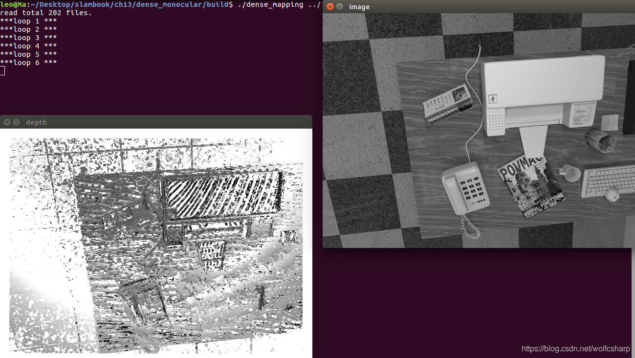
运行结果:
实验分析与讨论
像素梯度问题
有明显梯度的小块具有良好的区分度,不易引起误匹配,这反映了立体视觉对物体纹理的依赖性。
考虑两种极端的情况:像素梯度平行于极线方向,以及垂直于极线方向,如下图所示:
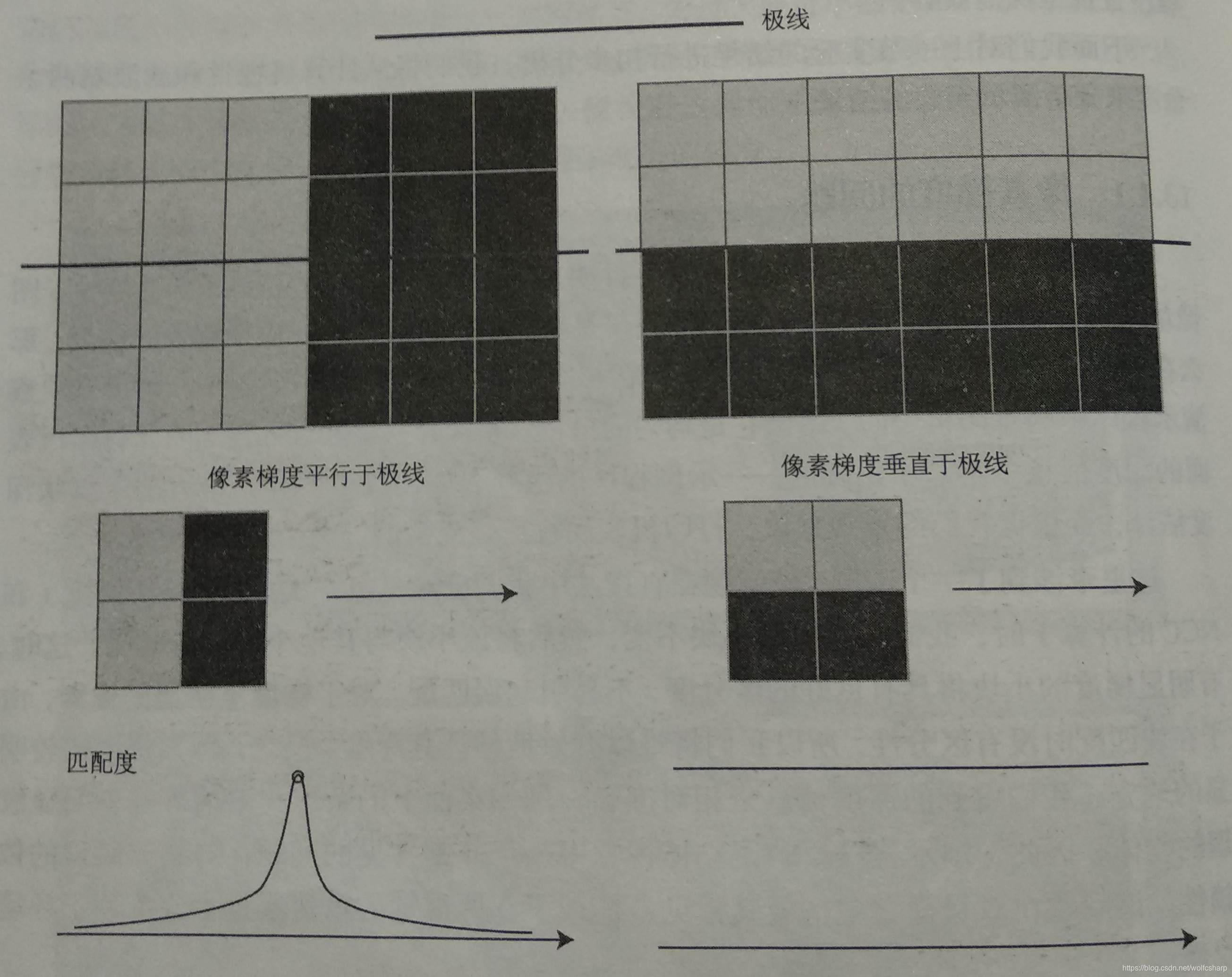
在垂直的情况下,即使小块有明显梯度,但沿着极线做块匹配时,会发现匹配程度都是一样的,因此得不到有效的匹配。
在平行的情况下,我们能够精确地确定匹配度最高点出现在何处。
实际当中,梯度与极线方向更可能不完全平行也不完全垂直。这时,我们说,当像素梯度与极线夹角较大时,极线匹配的不确定性大,当夹角较小时,匹配的不确定性变小。
逆深度
仿真发现。假设深度的倒数,也就是逆深度,为高斯分布是比较有效的。在实际应用中,逆深度也具有良好的数值稳定性,从而逐渐成为一种通用的技巧。
图像间的变换
块匹配假设了图像小块在相机运动时保持不变,但当相机发生明显的旋转是,就难以继续保持了。特别地,当相机绕光心旋转时,一块下黑上白的图像可能会变成一个上黑下白的图像块,导致相关性直接变成了负数(尽管仍然是同样一个块)。
为了防止这种情况的出现,我们通常需要在块匹配之前,把参考帧与当前帧之间的运动考虑进来。
根据相机模型,参考帧上的一个像素PR与真实的三维点世界坐标PW有以下关系:
dRPR = K(RRWPW+tRW)
对于当前帧,也有PW在它上面的投影,记作PC:
dCPC=K(RCWPW+tCW)
带入并消去PW,得到两幅图像之间的像素关系:
dCPC = dRKRCWRRWTK-1PR + Ktcw - KRCWRRWTKtRW
当知道dR,PR时,可以计算出PC的投影位置。此时,再给PR两个分量各一个增量du,dv,就可以求得PC的增量duc,dvc.通过这种方式,算出在局部范围内参考帧和当前帧图像坐标变换的一个线性关系构成仿射变换:
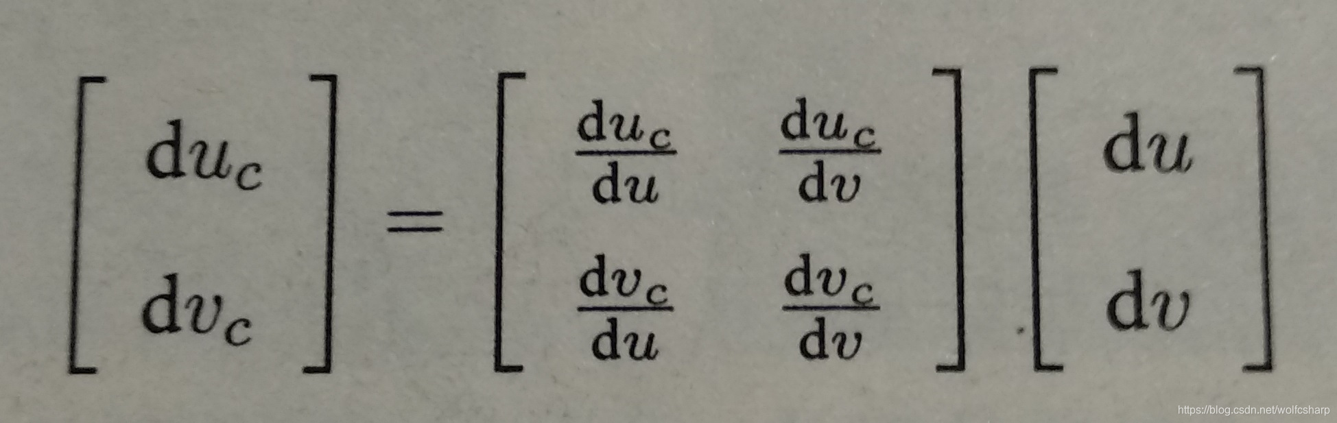
根据仿射变换矩阵,我们可以把当前帧(或参考帧)的像素进行变换后再进行块匹配,以期获得对旋转更好的效果。
RGB-D稠密建图
实践:点云地图
-
编译原书中pointcloud_mapping.cpp代码,运行时报错:
 参考文章https://blog.youkuaiyun.com/luanfei3717/article/details/80268597
解决办法:
在该程序中,加上头文件<Eigen/StdVector>,并将所有
std::vectorEigen::×× 都改为:
std::vector<Eigen::××,Eigen::aligned_allocatorEigen::××> -
完整代码
pointcloud_mapping.cpp
#include <iostream>
#include <fstream>
using namespace std;
#include <opencv2/core/core.hpp>
#include <opencv2/highgui/highgui.hpp>
#include <Eigen/Geometry>
#include <Eigen/StdVector> //这是后加的头文件
#include <boost/format.hpp> // for formating strings
#include <pcl/point_types.h>
#include <pcl/io/pcd_io.h>
#include <pcl/filters/voxel_grid.h>
//#include <pcl/visualization/pcl_visualizer.h> //这是后注释掉的头文件
#include <pcl/filters/statistical_outlier_removal.h>
int main( int argc, char** argv )
{
vector<cv::Mat> colorImgs, depthImgs; // 彩色图和深度图
vector<Eigen::Isometry3d,Eigen::aligned_allocator<Eigen::Isometry3d>> poses; //后修改的内容
//vector<Eigen::Isometry3d> poses; // 相机位姿
ifstream fin("../../data/pose.txt");
if (!fin)
{
cerr<<"cannot find pose file"<<endl;
return 1;
}
for ( int i=0; i<5; i++ )
{
boost::format fmt( "../../data/%s/%d.%s" ); //图像文件格式
colorImgs.push_back( cv::imread( (fmt%"color"%(i+1)%"png").str() ));
depthImgs.push_back( cv::imread( (fmt%"depth"%(i+1)%"pgm").str(), -1 )); // 使用-1读取原始图像
double data[7] = {0};
for ( int i=0; i<7; i++ )
{
fin>>data[i];
}
Eigen::Quaterniond q( data[6], data[3], data[4], data[5] );
Eigen::Isometry3d T(q);
T.pretranslate( Eigen::Vector3d( data[0], data[1], data[2] ));
poses.push_back( T );
}
// 计算点云并拼接
// 相机内参
double cx = 325.5;
double cy = 253.5;
double fx = 518.0;
double fy = 519.0;
double depthScale = 1000.0;
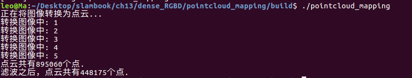
cout<<"正在将图像转换为点云..."<<endl;
// 定义点云使用的格式:这里用的是XYZRGB
typedef pcl::PointXYZRGB PointT;
typedef pcl::PointCloud<PointT> PointCloud;
// 新建一个点云
PointCloud::Ptr pointCloud( new PointCloud );
for ( int i=0; i<5; i++ )
{
PointCloud::Ptr current( new PointCloud );
cout<<"转换图像中: "<<i+1<<endl;
cv::Mat color = colorImgs[i];
cv::Mat depth = depthImgs[i];
Eigen::Isometry3d T = poses[i];
for ( int v=0; v<color.rows; v++ )
for ( int u=0; u<color.cols; u++ )
{
unsigned int d = depth.ptr<unsigned short> ( v )[u]; // 深度值
if ( d==0 ) continue; // 为0表示没有测量到
if ( d >= 7000 ) continue; // 深度太大时不稳定,去掉
Eigen::Vector3d point;
point[2] = double(d)/depthScale;
point[0] = (u-cx)*point[2]/fx;
point[1] = (v-cy)*point[2]/fy;
Eigen::Vector3d pointWorld = T*point;
PointT p ;
p.x = pointWorld[0];
p.y = pointWorld[1];
p.z = pointWorld[2];
p.b = color.data[ v*color.step+u*color.channels() ];
p.g = color.data[ v*color.step+u*color.channels()+1 ];
p.r = color.data[ v*color.step+u*color.channels()+2 ];
current->points.push_back( p );
}
// depth filter and statistical removal
PointCloud::Ptr tmp ( new PointCloud );
pcl::StatisticalOutlierRemoval<PointT> statistical_filter;
statistical_filter.setMeanK(50);
statistical_filter.setStddevMulThresh(1.0);
statistical_filter.setInputCloud(current);
statistical_filter.filter( *tmp );
(*pointCloud) += *tmp;
}
pointCloud->is_dense = false;
cout<<"点云共有"<<pointCloud->size()<<"个点."<<endl;
// voxel filter
pcl::VoxelGrid<PointT> voxel_filter;
voxel_filter.setLeafSize( 0.01, 0.01, 0.01 ); // resolution
PointCloud::Ptr tmp ( new PointCloud );
voxel_filter.setInputCloud( pointCloud );
voxel_filter.filter( *tmp );
tmp->swap( *pointCloud );
cout<<"滤波之后,点云共有"<<pointCloud->size()<<"个点."<<endl;
pcl::io::savePCDFileBinary("map.pcd", *pointCloud );
return 0;
}
CMakeLists.txt
cmake_minimum_required( VERSION 2.8 )

set( CMAKE_BUILD_TYPE Release )
set( CMAKE_CXX_FLAGS "-std=c++11" )

# opencv
find_package( OpenCV REQUIRED )
include_directories( ${OpenCV_INCLUDE_DIRS} )

# eigen
include_directories( "/usr/include/eigen3/" )

# pcl
find_package( PCL REQUIRED COMPONENT common io filters )
include_directories( ${PCL_INCLUDE_DIRS} )
add_definitions( ${PCL_DEFINITIONS} )

# octomap
#find_package( octomap REQUIRED )
#include_directories( ${OCTOMAP_INCLUDE_DIRS} )

add_executable( pointcloud_mapping pointcloud_mapping.cpp )
target_link_libraries( pointcloud_mapping ${OpenCV_LIBS} ${PCL_LIBRARIES} )

#add_executable( octomap_mapping octomap_mapping.cpp )
#target_link_libraries( octomap_mapping ${OpenCV_LIBS} ${PCL_LIBRARIES} ${OCTOMAP_LIBRARIES} )
3.运行结果
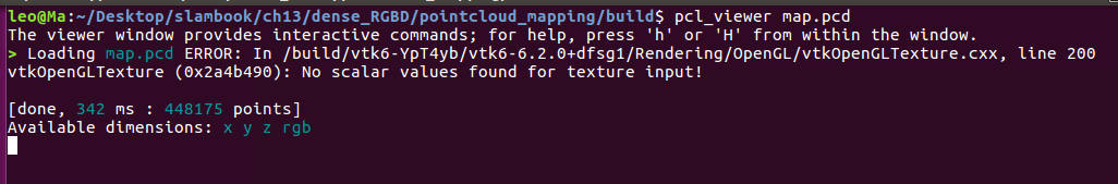
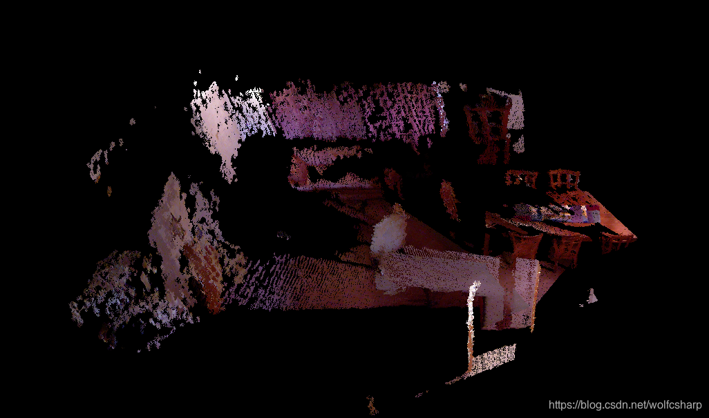
 得到map.pcd文件,用pcl_viewer打开它
pcl_viewer map.pcd
实践:八叉树地图
- 安装依赖
sudo apt-get install doxygen
- 安装octomap库
下载地址:https://github.com/OctoMap/octomap
它是一个cmake工程,编译安装即可。 - 完整代码
octomap_mapping.cpp
#include <iostream>
#include <fstream>
using namespace std;
#include <opencv2/core/core.hpp>
#include <opencv2/highgui/highgui.hpp>
#include <octomap/octomap.h> // for octomap
#include <Eigen/Geometry>
#include <boost/format.hpp> // for formating strings
int main( int argc, char** argv )
{
vector<cv::Mat> colorImgs, depthImgs; // 彩色图和深度图
vector<Eigen::Isometry3d> poses; // 相机位姿
ifstream fin("../../data/pose.txt");
if (!fin)
{
cerr<<"cannot find pose file"<<endl;
return 1;
}
for ( int i=0; i<5; i++ )
{
boost::format fmt( "../../data/%s/%d.%s" ); //图像文件格式
colorImgs.push_back( cv::imread( (fmt%"color"%(i+1)%"png").str() ));
depthImgs.push_back( cv::imread( (fmt%"depth"%(i+1)%"pgm").str(), -1 )); // 使用-1读取原始图像
double data[7] = {0};
for ( int i=0; i<7; i++ )
{
fin>>data[i];
}
Eigen::Quaterniond q( data[6], data[3], data[4], data[5] );
Eigen::Isometry3d T(q);
T.pretranslate( Eigen::Vector3d( data[0], data[1], data[2] ));
poses.push_back( T );
}
// 计算点云并拼接
// 相机内参
double cx = 325.5;
double cy = 253.5;
double fx = 518.0;
double fy = 519.0;
double depthScale = 1000.0;
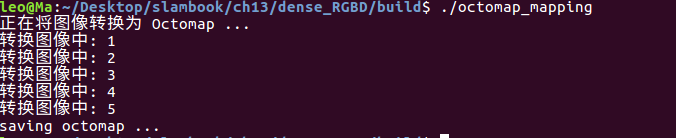
cout<<"正在将图像转换为 Octomap ..."<<endl;
// octomap tree
octomap::OcTree tree( 0.05 ); // 参数为分辨率
for ( int i=0; i<5; i++ )
{
cout<<"转换图像中: "<<i+1<<endl;
cv::Mat color = colorImgs[i];
cv::Mat depth = depthImgs[i];
Eigen::Isometry3d T = poses[i];
octomap::Pointcloud cloud; // the point cloud in octomap
for ( int v=0; v<color.rows; v++ )
for ( int u=0; u<color.cols; u++ )
{
unsigned int d = depth.ptr<unsigned short> ( v )[u]; // 深度值
if ( d==0 ) continue; // 为0表示没有测量到
if ( d >= 7000 ) continue; // 深度太大时不稳定,去掉
Eigen::Vector3d point;
point[2] = double(d)/depthScale;
point[0] = (u-cx)*point[2]/fx;
point[1] = (v-cy)*point[2]/fy;
Eigen::Vector3d pointWorld = T*point;
// 将世界坐标系的点放入点云
cloud.push_back( pointWorld[0], pointWorld[1], pointWorld[2] );
}
// 将点云存入八叉树地图,给定原点,这样可以计算投射线
tree.insertPointCloud( cloud, octomap::point3d( T(0,3), T(1,3), T(2,3) ) );
}
// 更新中间节点的占据信息并写入磁盘
tree.updateInnerOccupancy();
cout<<"saving octomap ... "<<endl;
tree.writeBinary( "octomap.bt" );
return 0;
}
CMakeLists.txt
cmake_minimum_required( VERSION 2.8 )

set( CMAKE_BUILD_TYPE Release )
set( CMAKE_CXX_FLAGS "-std=c++11" )

# opencv
find_package( OpenCV REQUIRED )
include_directories( ${OpenCV_INCLUDE_DIRS} )

# eigen
include_directories( "/usr/include/eigen3/" )

# pcl
#find_package( PCL REQUIRED COMPONENT common io filters )
#include_directories( ${PCL_INCLUDE_DIRS} )
#add_definitions( ${PCL_DEFINITIONS} )

# octomap
find_package( octomap REQUIRED )
include_directories( ${OCTOMAP_INCLUDE_DIRS} )

#add_executable( pointcloud_mapping pointcloud_mapping.cpp )
#target_link_libraries( pointcloud_mapping ${OpenCV_LIBS} ${PCL_LIBRARIES} )

add_executable( octomap_mapping octomap_mapping.cpp )
target_link_libraries( octomap_mapping ${OpenCV_LIBS} ${PCL_LIBRARIES} ${OCTOMAP_LIBRARIES} )
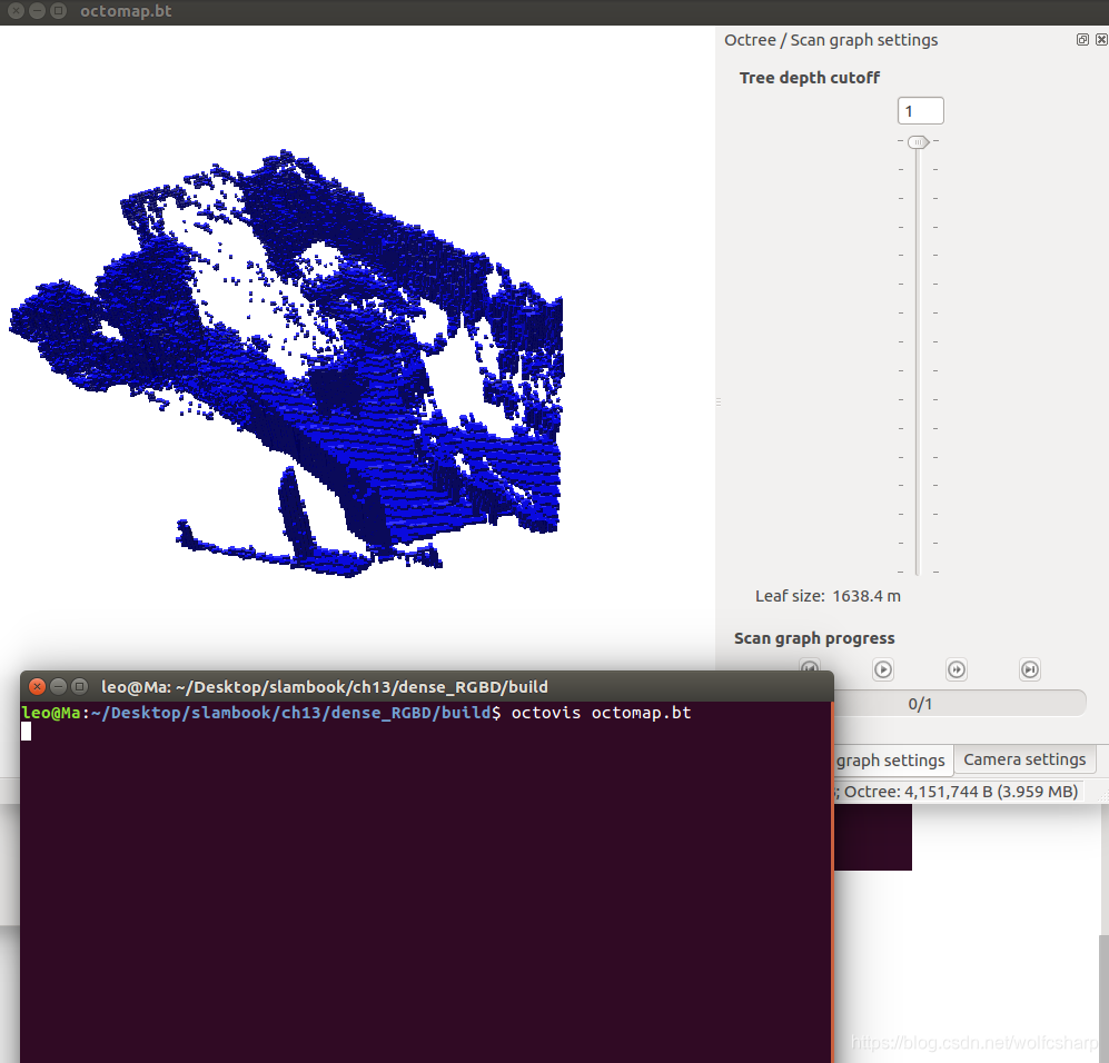
- 运行结果


 506
506

 被折叠的 条评论
为什么被折叠?
被折叠的 条评论
为什么被折叠?
 到【灌水乐园】发言


