


概要:在本文中,我将介绍图形数据集Cora,同时利用Gephi处理数据集中的节点特征。之后,我们尝试在神经网络中包含拓扑信息(topological infomation),并比较加入拓扑信息前后的神经网络的性能。
一、Cora数据集介绍
Cora数据集包括2708份科学出版物,分为7类。引文网络由5429个链接组成。数据集中的每个发布都用一个0/1值的词向量来描述,该词向量表示字典中相应词的缺失/存在。这部词典由1433个独特的单词组成。


提示:以下是本篇文章正文内容,下面案例可供参考
二、GNN架构
理解GNN架构首先需要理解多层感知机(MLP)在简单线性层的定义。
一个基本的神经网络对应于一个线性变换:
h
A
=
x
A
W
T
h_A=x_AW^T
hA=xAWT
式中,
x
A
x_A
xA是输入的节点向量,
W
W
W是权重矩阵。
对于图数据集,输入向量是节点特征,这意味着节点之间是完全分离的。但是,我们需要考虑节点的上下文对节点的作用。因此,我们需要查看节点的邻域来帮助我们更好的进行节点分类。
定义
N
A
N_A
NA为节点
A
A
A的邻域。进而,我们图线性变换层可以写为:
h
A
=
∑
i
∈
N
A
x
i
W
T
h_A=\sum_{i\in N_A}{x_iW^T}
hA=i∈NA∑xiWT
将其转变为神经网络的矩阵运算格式,则为:
H
=
A
~
T
X
W
T
H=\tilde{A}^TXW^T
H=A~TXWT
式中:
A
~
=
A
+
I
\tilde{A}=A+I
A~=A+I 表示邻接矩阵和自循环矩阵之和。
三、代码解析
首先,我们利用MLP架构对节点进行分类。之后,利用GNN架构进行分类,并比较加入邻接矩阵前后模型的性能。
1、数据库导入
import torch
import torch.nn.functional as F
import pandas as pd
import csv
from torch.nn import Linear
from torch_geometric.datasets import Planetoid
from torch_geometric.datasets import FacebookPagePage
from torch_geometric.utils import to_dense_adj

torch.manual_seed(0)
2、MLP架构
定义准确度函数以及构建MLP架构。
# Model Create
def accuracy(y_pred, y_true):
    """Calculate accuracy."""
    return torch.sum(y_pred == y_true) / len(y_true)


class MLP(torch.nn.Module):
    """Multilayer Perceptron"""
    # the number of neurons in the input, hidden and output layers
    def __init__(self, dim_in, dim_h, dim_out):
        super().__init__()
        self.linear1 = Linear(dim_in, dim_h)
        self.linear2 = Linear(dim_h, dim_out)

    def forward(self, x):
        x = self.linear1(x)
        x = torch.relu(x)
        x = self.linear2(x)
        return F.log_softmax(x, dim=1)

    def fit(self, data, epochs):
        # initialize a loss function and an optimizer
        criterion = torch.nn.CrossEntropyLoss()
        optimizer = torch.optim.Adam(self.parameters(),
                                          lr=0.01,
                                          weight_decay=5e-4)

        self.train()

        losses = []
        accs = []
        val_losses = []
        val_accs = []
        for epoch in range(epochs+1):
            optimizer.zero_grad()
            out = self(data.x)
            loss = criterion(out[data.train_mask], data.y[data.train_mask])
            acc = accuracy(out[data.train_mask].argmax(dim=1),
                          data.y[data.train_mask])
            loss.backward()
            optimizer.step()

            losses.append(loss)
            accs.append(acc)

            val_loss = criterion(out[data.val_mask], data.y[data.val_mask])
            val_acc = accuracy(out[data.val_mask].argmax(dim=1),
                              data.y[data.val_mask])
            print(f'Epoch {epoch:>3} | Train Loss: {loss:.3f} | Train Acc:'
                  f' {acc*100:>5.2f}% | Val Loss: {val_loss:.2f} | '
                  f'Val Acc: {val_acc*100:.2f}%')

            val_losses.append(val_loss)
            val_accs.append(val_acc)

        self.train_loss = losses
        self.train_acc = accs
        self.val_loss = val_losses
        self.val_acc = val_accs

    @torch.no_grad()
    def test(self, data):
        self.eval()
        out = self(data.x)
        acc = accuracy(out.argmax(dim=1)[data.test_mask], data.y[data.test_mask])
        return acc
在上述MLP类中,首先初始化了两层线性层,并分别定义了它们的输入输出大小。其次在 f o r w a r d forward forward函数中,分别定义激活函数为 r e l u relu relu和 l o g _ s o f t m a x log\_softmax log_softmax,最后在 f i t fit fit函数中,定义了损失函数和优化器。
3、训练MLP模型
# Create MLP model
mlp = MLP(dataset.num_features, 16, dataset.num_classes)
print(mlp)

# Train
mlp.fit(data, epochs=100)

# Test
acc = mlp.test(data)
print(f'\nMLP test accuracy: {acc*100:.2f}%')

# plot
plt.plot(range(101), np.array(mlp.train_loss), label="Training loss")
plt.plot(range(101), np.array(mlp.val_loss), ":", label="Val loss")
plt.title("Training and validation loss")
plt.style.use('seaborn-colorblind')
plt.xlabel("Epochs")
plt.ylabel("Loss")
plt.legend()
plt.show()

plt.plot(range(101), np.array(mlp.train_acc), label="Training acc")
plt.plot(range(101), np.array(mlp.val_acc), ':', label="Val acc")
plt.style.use('seaborn-colorblind')
plt.title("Training and validation acc")
plt.xlabel("Epochs")
plt.ylabel("acc")
plt.legend()
plt.show()
保存训练过程中的
l
o
s
s
loss
loss和
a
c
c
acc
acc以便于可视化,通过观察验证集
l
o
s
s
loss
loss和
a
c
c
acc
acc的变化防止过拟合的发生。
训练后得到的结果如图3所示:
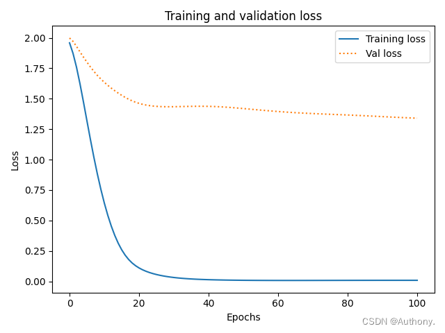
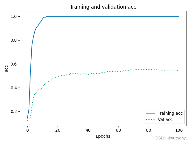
从图3中可以看出,MLP架构的训练结果较差,验证集的准确率只能达到45%,同时在训练次数达到18次左右的时候,训练集的准确率就不在变化。
综上,模型在一定程度上有过拟合的现象发生,模型参数在后续的训练中变化幅度较小。
4、GNN架构
首先建立GNN架构中关于邻接矩阵运算的函数。
class VanillaGNNLayer(torch.nn.Module):
    def __init__(self, dim_in, dim_out):
        super().__init__()
        # bias=False: which means without bias
        self.linear = Linear(dim_in, dim_out, bias=False)

    def forward(self, x, adjacency):
        x = self.linear(x)
        x = torch.sparse.mm(adjacency, x)
        return x


# adjacency matrix
# The two lines correspond one to one
# [[[ ]]] --> [0] --> [[ ]]
adjacency = to_dense_adj(data.edge_index)[0]
# self loops
# sparse matrix
adjacency += torch.eye(len(adjacency))
在上述类中,我们构建了线性模型,并将线性偏置去除,同时用
t
o
r
c
h
.
s
p
a
r
s
e
.
m
m
torch.sparse.mm
torch.sparse.mm将邻接矩阵加入到运算中。
在程序运行部分,我们用
t
o
r
c
h
torch
torch中的
t
o
_
d
e
n
s
e
_
a
d
j
to\_dense\_adj
to_dense_adj函数将相邻节点的对应关系转化为邻接矩阵的形式,并且通过
e
y
e
eye
eye函数引入自循环。
GNN模型的建立
class VanillaGNN(torch.nn.Module):
    """Vanilla Graph Neural Network"""
    def __init__(self, dim_in, dim_h, dim_out):
        super().__init__()
        # without bias and connect the adjacency matrix
        self.gnn1 = VanillaGNNLayer(dim_in, dim_h)
        self.gnn2 = VanillaGNNLayer(dim_h, dim_out)

    def forward(self, x, adjacency):
        h = self.gnn1(x, adjacency)
        h = torch.relu(h)
        h = self.gnn2(h, adjacency)
        return F.log_softmax(h, dim=1)

    def fit(self, data, epochs):
        criterion = torch.nn.CrossEntropyLoss()
        optimizer = torch.optim.Adam(self.parameters(),
                                      lr=0.01,
                                      weight_decay=5e-4)

        self.train()
        losses = []
        accs = []
        val_losses = []
        val_accs = []

        for epoch in range(epochs+1):
            optimizer.zero_grad()
            out = self(data.x, adjacency)
            loss = criterion(out[data.train_mask], data.y[data.train_mask])
            acc = accuracy(out[data.train_mask].argmax(dim=1),
                          data.y[data.train_mask])
            loss.backward()
            optimizer.step()

            val_loss = criterion(out[data.val_mask], data.y[data.val_mask])
            val_acc = accuracy(out[data.val_mask].argmax(dim=1),
                              data.y[data.val_mask])
            print(f'Epoch {epoch:>3} | Train Loss: {loss:.3f} | Train Acc:'
                  f' {acc*100:>5.2f}% | Val Loss: {val_loss:.2f} | '
                  f'Val Acc: {val_acc*100:.2f}%')

            losses.append(loss)
            accs.append(acc)
            val_losses.append(val_loss)
            val_accs.append(val_acc)

        self.train_loss = losses
        self.train_acc = accs
        self.val_loss = val_losses
        self.val_acc = val_accs

    @torch.no_grad()
    def test(self, data):
        self.eval()
        out = self(data.x, adjacency)
        acc = accuracy(out.argmax(dim=1)[data.test_mask], data.y[data.test_mask])
        return acc
GNN模型同MLP模型相类似,在此不多赘述。
5、训练GNN模型
# Create the Vanilla GNN model
gnn = VanillaGNN(dataset.num_features, 16, dataset.num_classes)
print(gnn)

# Train
gnn.fit(data, epochs=100)

# Test
acc = gnn.test(data)
print(f'\nGNN test accuracy: {acc*100:.2f}%')

# plot
plt.plot(range(101), np.array(gnn.train_loss), label="Training loss")
plt.plot(range(101), np.array(gnn.val_loss), ":", label="Val loss")
plt.title("GNN Training and validation loss")
plt.style.use('seaborn-colorblind')
plt.xlabel("Epochs")
plt.ylabel("Loss")
plt.legend()
plt.show()

plt.plot(range(101), np.array(gnn.train_acc), label="Training acc")
plt.plot(range(101), np.array(gnn.val_acc), ':', label="Val acc")
plt.style.use('seaborn-colorblind')
plt.title("GNN Training and validation acc")
plt.xlabel("Epochs")
plt.ylabel("acc")
plt.legend()
plt.show()
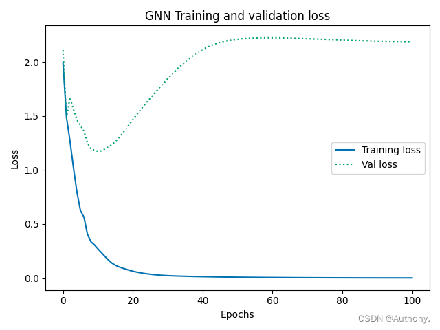
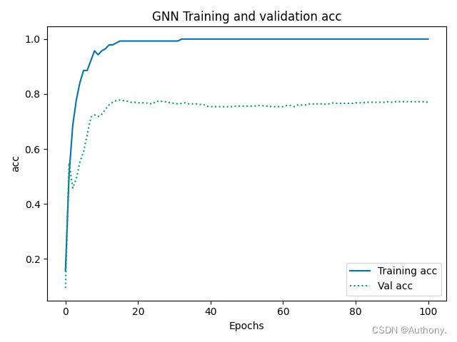
模型训练结果如图4所示:
6、Tensorflow库
前文的MLP模型,我们采用 t o r c h torch torch库中关于神经网络的架构。在此,我们更改为 t e n s o r f l o w tensorflow tensorflow库,比较模型的结果。
# 二分类用交叉熵作为损失函数
model.compile(optimizer="rmsprop",
              loss="categorical_crossentropy",
              metrics=["accuracy"])

# 训练模型
history = model.fit(X_train,
                    y_train,
                    epochs=40,
                    batch_size=128,
                    validation_data=(X_val, y_val))
上述是
t
e
n
s
o
r
f
l
o
w
tensorflow
tensorflow神经网络模型的主要架构。
模型的训练结果如图5所示:
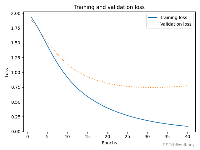
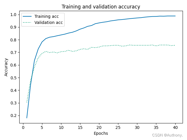
从图5中我们可以看出,同样是MLP模型,利用
t
e
n
s
o
r
f
l
o
w
tensorflow
tensorflow库训练的神经网络其验证集的准确率可以达到70%。
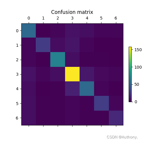
利用上述训练好的模型可以得到测试集的混淆矩阵如图6所示。
总结
在本章中,我们了解了MLP和GNN之间不同的环节。我们用我们的直觉和一点线性代数建立了我们自己的GNN架构。我们从科学文献中探索了流行的图数据集来比较我们的两种架构。最后,我们在Python中实现了它们,并评估了它们的性能。


 1万+
1万+

 被折叠的 条评论
为什么被折叠?
被折叠的 条评论
为什么被折叠?
 到【灌水乐园】发言


