


弱监督学习文献解读:Transformer based multiple instance learning for weakly supervised histopathology image segmentation
原文地址:https://arxiv.org/pdf/2205.08878.pdf
后续会添加代码解读
在MIL中,一个包(bag)表示一个含有多个实例的集合,而不是将每个实例都视为独立的。包级别的分类任务是确定整个包属于哪个类别。在这项工作中,是否癌变的图像被视为包,而图像中的像素被视为实例。****深度监督****通过在网络的多个中间层引入额外的损失函数,从而提供了更多的梯度信号。
文章优点
提出了一种基于变压器的弱监督语义分割方法。在框架中利用深度监督来利用多尺度特征并提供更多的监督信息。
方法
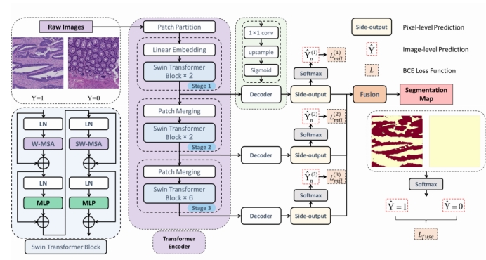
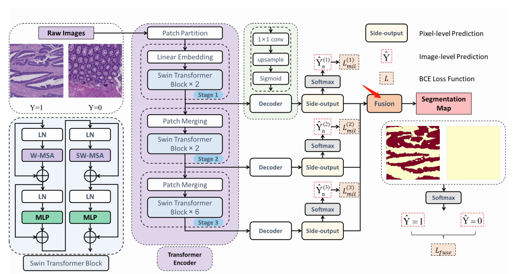
Swin-MIL由Swin变压器编码器、解码器和深度监督组成。Swin变压器编码器在分配注意力权重的特征中发挥着重要作用。通过捕获全局信息,自我注意模块有效地突出了在每个阶段具有更好的可解释性的特征。每个阶段的解码器生成像素级的预测作为侧输出,其中最终的分割图与所有阶段的侧输出融合。
Swin Transformer encoder
首先将图像Xn裁剪成不重叠的补丁,补丁大小为4×4。每个补丁被视为一个“令牌”,输入几个Swin变压器块,通过多头自注意增强特征图中的重要区域,并通过多头自注意抑制无关区域的影响。Swin变压器块以及一个线性嵌入层被称为“阶段1”,它将原始值特征投射到任意维数上。为了生成多尺度的特征表示,随着网络的深入,引入了补丁合并层来减少标记的数量。第二阶段和第三阶段输出像素分别为原始图像长宽的八分之一和十六分之一。
swin Transformer代码
class SwinTransformerBlock(nn.Module):
    """ Swin Transformer Block.

    Args:
        dim (int): Number of input channels.
        num_heads (int): Number of attention heads.
        window_size (int): Window size.
        shift_size (int): Shift size for SW-MSA.
        mlp_ratio (float): Ratio of mlp hidden dim to embedding dim.
        qkv_bias (bool, optional): If True, add a learnable bias to query, key, value. Default: True
        qk_scale (float | None, optional): Override default qk scale of head_dim ** -0.5 if set.
        drop (float, optional): Dropout rate. Default: 0.0
        attn_drop (float, optional): Attention dropout rate. Default: 0.0
        drop_path (float, optional): Stochastic depth rate. Default: 0.0
        act_layer (nn.Module, optional): Activation layer. Default: nn.GELU
        norm_layer (nn.Module, optional): Normalization layer.  Default: nn.LayerNorm
    """

    def __init__(self, dim, num_heads, window_size=7, shift_size=0,
                 mlp_ratio=4., qkv_bias=True, qk_scale=None, drop=0., attn_drop=0., drop_path=0.,
                 act_layer=nn.GELU, norm_layer=nn.LayerNorm):
        super().__init__()
        self.dim = dim
        self.num_heads = num_heads
        self.window_size = window_size
        self.shift_size = shift_size
        self.mlp_ratio = mlp_ratio
        assert 0 <= self.shift_size < self.window_size, "shift_size must in 0-window_size"

        self.norm1 = norm_layer(dim)
        self.attn = WindowAttention(
            dim, window_size=to_2tuple(self.window_size), num_heads=num_heads,
            qkv_bias=qkv_bias, qk_scale=qk_scale, attn_drop=attn_drop, proj_drop=drop)

        self.drop_path = DropPath(drop_path) if drop_path > 0. else nn.Identity()
        self.norm2 = norm_layer(dim)
        mlp_hidden_dim = int(dim * mlp_ratio)
        self.mlp = Mlp(in_features=dim, hidden_features=mlp_hidden_dim, act_layer=act_layer, drop=drop)

        self.H = None
        self.W = None

    def forward(self, x, mask_matrix):
        """ Forward function.

        Args:
            x: Input feature, tensor size (B, H*W, C).
            H, W: Spatial resolution of the input feature.
            mask_matrix: Attention mask for cyclic shift.
        """
        B, L, C = x.shape
        H, W = self.H, self.W
        assert L == H * W, "input feature has wrong size"

        shortcut = x
        x = self.norm1(x)
        x = x.view(B, H, W, C)

        # pad feature maps to multiples of window size
        pad_l = pad_t = 0
        pad_r = (self.window_size - W % self.window_size) % self.window_size
        pad_b = (self.window_size - H % self.window_size) % self.window_size
        x = F.pad(x, (0, 0, pad_l, pad_r, pad_t, pad_b))
        _, Hp, Wp, _ = x.shape

        # cyclic shift
        if self.shift_size > 0:
            shifted_x = torch.roll(x, shifts=(-self.shift_size, -self.shift_size), dims=(1, 2))
            attn_mask = mask_matrix
        else:
            shifted_x = x
            attn_mask = None

        # partition windows
        x_windows = window_partition(shifted_x, self.window_size)  # nW*B, window_size, window_size, C
        x_windows = x_windows.view(-1, self.window_size * self.window_size, C)  # nW*B, window_size*window_size, C

        # W-MSA/SW-MSA
        attn_windows = self.attn(x_windows, mask=attn_mask)  # nW*B, window_size*window_size, C

        # merge windows
        attn_windows = attn_windows.view(-1, self.window_size, self.window_size, C)
        shifted_x = window_reverse(attn_windows, self.window_size, Hp, Wp)  # B H' W' C

        # reverse cyclic shift
        if self.shift_size > 0:
            x = torch.roll(shifted_x, shifts=(self.shift_size, self.shift_size), dims=(1, 2))
        else:
            x = shifted_x

        if pad_r > 0 or pad_b > 0:
            x = x[:, :H, :W, :].contiguous()

        x = x.view(B, H * W, C)

        # FFN
        x = shortcut + self.drop_path(x)
        x = x + self.drop_path(self.mlp(self.norm2(x)))

        return x
补丁融合阶段代码
class PatchMerging(nn.Module):
    """ Patch Merging Layer

    Args:
        dim (int): Number of input channels.
        norm_layer (nn.Module, optional): Normalization layer.  Default: nn.LayerNorm
    """
    def __init__(self, dim, norm_layer=nn.LayerNorm):
        super().__init__()
        self.dim = dim
        self.reduction = nn.Linear(4 * dim, 2 * dim, bias=False)
        self.norm = norm_layer(4 * dim)

    def forward(self, x, H, W):
        """ Forward function.

        Args:
            x: Input feature, tensor size (B, H*W, C).
            H, W: Spatial resolution of the input feature.
        """
        B, L, C = x.shape
        assert L == H * W, "input feature has wrong size"

        x = x.view(B, H, W, C)

        # padding
        pad_input = (H % 2 == 1) or (W % 2 == 1)
        if pad_input:
            x = F.pad(x, (0, 0, 0, W % 2, 0, H % 2))

        x0 = x[:, 0::2, 0::2, :]  # B H/2 W/2 C
        x1 = x[:, 1::2, 0::2, :]  # B H/2 W/2 C
        x2 = x[:, 0::2, 1::2, :]  # B H/2 W/2 C
        x3 = x[:, 1::2, 1::2, :]  # B H/2 W/2 C
        x = torch.cat([x0, x1, x2, x3], -1)  # B H/2 W/2 4*C
        x = x.view(B, -1, 4 * C)  # B H/2*W/2 4*C

        x = self.norm(x)
        x = self.reduction(x)

        return x
解码器部分
输出特征图的通道大小被1×1的卷积层压缩到1。经过双线性上采样(这部分可能改成转置卷积上采样等方法)操作后,它被恢复到原来的大小(H×W),最终被s型激活,生成一个预测的概率图作为侧输出。
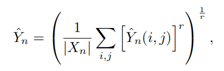
提出了一个融合层来充分利用所有阶段的多尺度侧输出来预测最终的分割图。
Y
n
ˆ
(
i
,
j
)
Y^ˆ_n(i, j)
Ynˆ(i,j)
表示第n幅图中(i,j)像素的值,使用 Generalized Mean (GM)的方法对图像进行处理(公式如下),得到
Y
n
ˆ
Y^ˆ_n
Ynˆ
即表示图像类别。
深度监督
为了解决MIL中监督信息缺失的问题,有效利用分层信息,我们引入了深度监督。
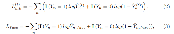
损失函数被定义为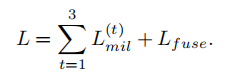
在每个侧输出和融合层中,损失函数以深度监督的形式计算,没有任何额外的像素级标签监督。然后,利用随机梯度下降算法,通过反向传播来最小化目标函数来学习参数。
算法效果
2kn-1684240728029)]
损失函数被定义为[外链图片转存中…(img-3hWkpwQz-1684240728029)]
在每个侧输出和融合层中,损失函数以深度监督的形式计算,没有任何额外的像素级标签监督。然后,利用随机梯度下降算法,通过反向传播来最小化目标函数来学习参数。
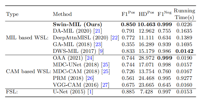
算法效果
[外链图片转存中…(img-HIAeDxMe-1684240728030)]
其中FSL表示全监督学习,WSL表示弱监督学习
初读本文献,若有理解不到位的地方欢迎大佬批评指正


 66
66

 被折叠的 条评论
为什么被折叠?
被折叠的 条评论
为什么被折叠?
 到【灌水乐园】发言


