


cs231n Assignment1
文章目录
前言
本文为 2024 年斯坦福 cs231n 作业一 的参考答案,代码框架可在官网下载,作业一包含 5 个问题:
- k-Nearest Neighbor classifier
- Training a Support Vector Machine
- Implement a Softmax classifier
- Two-Layer Neural Network
- Higher Level Representations: Image Features
Q1: k-Nearest Neighbor classifier
kNN 分类器由两个阶段组成:
- 在训练期间,分类器获取训练数据并简单记忆。
- 在测试阶段,kNN 将每张测试图像与所有训练图像进行比较,并将最相似的 k 个训练实例的标签进行投票,从而对图像进行分类。
- k 值经过交叉验证。
cs231n 作业使用的数据集为 CIFAR-10,数据集包含 60000 张共 10 个类别的 32x32x3 的彩色图片,每个类别共有 6000 张图片,训练集包含 50000 张图片,测试集包含 10000 张图片,数据集详细介绍可参考 CIFAR-10 数据集官网。

kNN 分类器的训练代码如下:
class KNearestNeighbor(object):
    """ a kNN classifier with L2 distance """

    def train(self, X, y):
        """
        Train the classifier. For k-nearest neighbors this is just
        memorizing the training data.

        Inputs:
        - X: A numpy array of shape (num_train, D) containing the training data
          consisting of num_train samples each of dimension D.
        - y: A numpy array of shape (N,) containing the training labels, where
             y[i] is the label for X[i].
        """
        self.X_train = X
        self.y_train = y
现在,我们想用 kNN 分类器对测试数据进行分类。我们可以将这一过程分为两个步骤:
- 首先,我们必须计算所有测试示例和所有训练示例之间的距离。
- 根据这些距离,我们为每个测试示例找出 k 个最近的示例,并让它们为标签投票,票数最高的标签即为预测结果。
compute_distances_two_loops
使用两重 for 循环,计算所有测试示例和所有训练示例之间的距离,距离指标采用 L2 距离(欧几里得距离):
d
2
(
I
1
p
,
I
2
p
)
=
∑
p
(
I
1
p
−
I
2
p
)
2
d_2(I_1^p,I_2^p)=\sqrt{\sum_p(I_1^p-I_2^p)^2}
d2(I1p,I2p)=p∑(I1p−I2p)2
dists[i, j] 表示第 i 个测试图片与第 j 个训练图片的距离,实现思路为:
- 遍历每一组测试图片和训练图片。
- 通过表达式
np.sqrt(np.sum(np.square(X[i] - self.X_train[j])))计算每一组图片的 L2 距离。
def compute_distances_two_loops(self, X):
    """
    Compute the distance between each test point in X and each training point
    in self.X_train using a nested loop over both the training data and the
    test data.

    Inputs:
    - X: A numpy array of shape (num_test, D) containing test data.

    Returns:
    - dists: A numpy array of shape (num_test, num_train) where dists[i, j]
      is the Euclidean distance between the ith test point and the jth training
      point.
    """
    num_test = X.shape[0]
    num_train = self.X_train.shape[0]
    dists = np.zeros((num_test, num_train))
    for i in range(num_test):
        for j in range(num_train):
            #####################################################################
            # TODO:                                                             #
            # Compute the l2 distance between the ith test point and the jth    #
            # training point, and store the result in dists[i, j]. You should   #
            # not use a loop over dimension, nor use np.linalg.norm().          #
            #####################################################################
            # *****START OF YOUR CODE (DO NOT DELETE/MODIFY THIS LINE)*****

            dists[i, j] = np.sqrt(np.sum(np.square(X[i] - self.X_train[j])))

            # *****END OF YOUR CODE (DO NOT DELETE/MODIFY THIS LINE)*****
    return dists
Inline Question 1:
请注意距离矩阵中的结构模式,其中某些行或列明显更亮。(请注意,在默认配色方案中,黑色表示距离小,白色表示距离大)。
- 在数据中,是什么原因导致这些行明显变亮?
- 是什么导致了这些列?
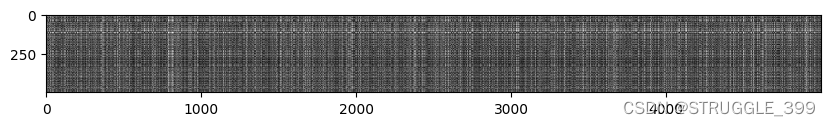
【答】距离矩阵某一行明显更亮说明对应的测试图片与所有训练图片的 L2 距离都很大,距离矩阵某一列明显更亮说明对应的训练图片与所有测试图片的 L2 距离都很大。
predict_labels
计算距离矩阵 dists 后,可以根据 dists 进行类别预测,实现思路为:
- 遍历距离矩阵
dists每一行。 - 获取距离最近的 k 个训练图片的标签,存放在列表
closest_y中。 - 将 k 个距离最近的训练图片标签进行投票,票数最高的标签为预测结果。
def predict_labels(self, dists, k=1):
    """
    Given a matrix of distances between test points and training points,
    predict a label for each test point.

    Inputs:
    - dists: A numpy array of shape (num_test, num_train) where dists[i, j]
      gives the distance betwen the ith test point and the jth training point.

    Returns:
    - y: A numpy array of shape (num_test,) containing predicted labels for the
      test data, where y[i] is the predicted label for the test point X[i].
    """
    num_test = dists.shape[0]
    y_pred = np.zeros(num_test)
    for i in range(num_test):
        # A list of length k storing the labels of the k nearest neighbors to
        # the ith test point.
        closest_y = []
        #########################################################################
        # TODO:                                                                 #
        # Use the distance matrix to find the k nearest neighbors of the ith    #
        # testing point, and use self.y_train to find the labels of these       #
        # neighbors. Store these labels in closest_y.                           #
        # Hint: Look up the function numpy.argsort.                             #
        #########################################################################
        # *****START OF YOUR CODE (DO NOT DELETE/MODIFY THIS LINE)*****

        closest_y = [self.y_train[i] for i in np.argsort(dists[i, :])[:k]]

        # *****END OF YOUR CODE (DO NOT DELETE/MODIFY THIS LINE)*****
        #########################################################################
        # TODO:                                                                 #
        # Now that you have found the labels of the k nearest neighbors, you    #
        # need to find the most common label in the list closest_y of labels.   #
        # Store this label in y_pred[i]. Break ties by choosing the smaller     #
        # label.                                                                #
        #########################################################################
        # *****START OF YOUR CODE (DO NOT DELETE/MODIFY THIS LINE)*****

        count = np.zeros(10)
        most_common_label, maxcount = -1, -1
        for label in closest_y:
          count[label] += 1
          if count[label] > maxcount:
            maxcount = count[label]
            most_common_label = label
        y_pred[i] = most_common_label

        # *****END OF YOUR CODE (DO NOT DELETE/MODIFY THIS LINE)*****
    return y_pred
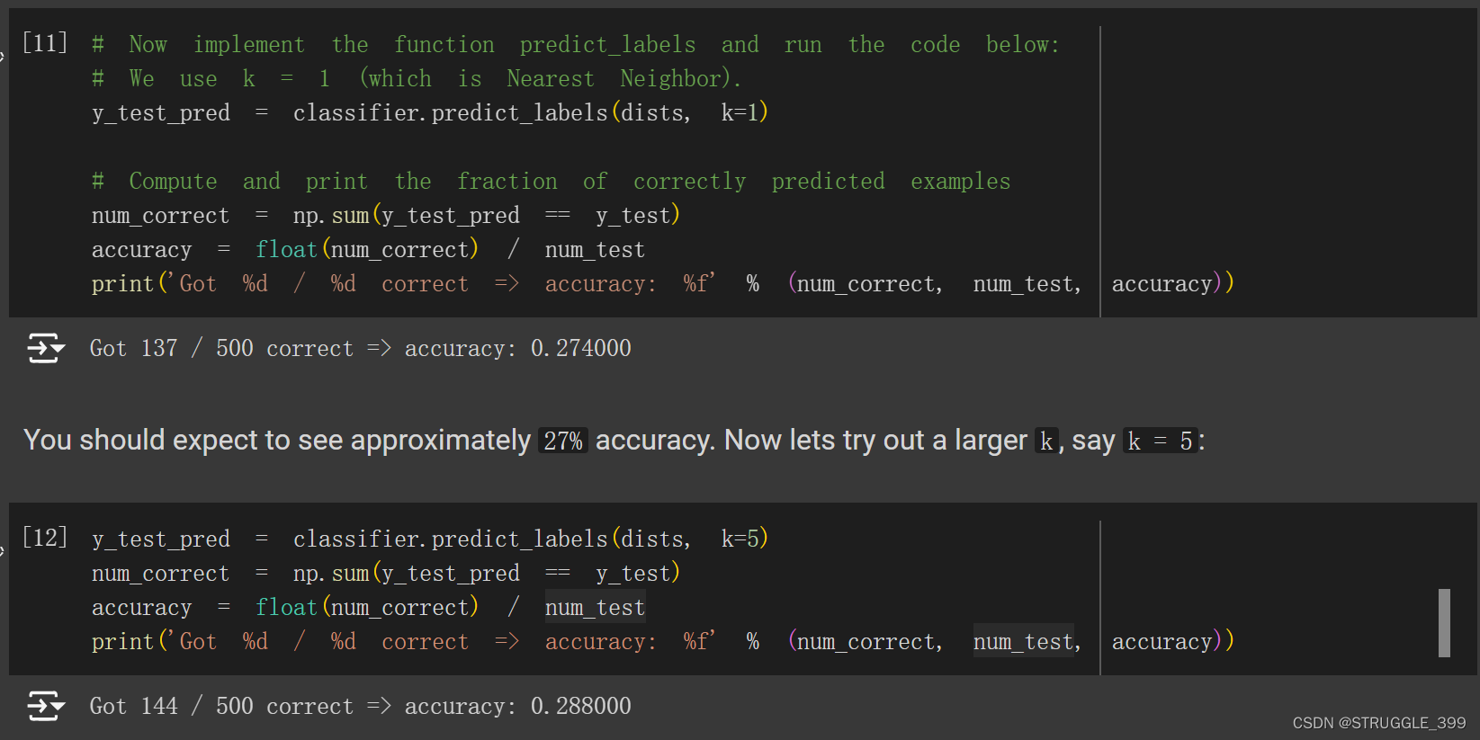
predict_labels 实现完成后,对 k=1 和 k=5 两种情况进行测试,分别得到的测试精度为 0.274、0.288。
Inline Question 2:
我们还可以使用其他距离指标,如 L1 距离。记
p
i
j
(
k
)
p_{ij}^{(k)}
pij(k) 为图片
I
k
I_k
Ik 在位置
(
i
,
j
)
(i,j)
(i,j) 处的像素值,所有图片的所有像素均值
μ
\mu
μ 为:
μ
=
1
n
h
w
∑
k
=
1
n
∑
i
=
1
h
∑
j
=
1
w
p
i
j
(
k
)
\mu=\frac{1}{nhw}\sum_{k=1}^n\sum_{i=1}^h\sum_{j=1}^wp_{ij}^{(k)}
μ=nhw1k=1∑ni=1∑hj=1∑wpij(k)
所有图像的像素平均值
μ
i
j
\mu_{ij}
μij 为:
μ
i
j
=
1
n
∑
k
=
1
n
p
i
j
(
k
)
\mu_{ij}=\frac{1}{n}\sum_{k=1}^n p_{ij}^{(k)}
μij=n1k=1∑npij(k)
所有图片的所有像素标准差
σ
\sigma
σ 和所有图像的像素标准差
σ
i
j
\sigma_{ij}
σij 的定义是类似的。
以下哪些预处理步骤不会改变使用 L1 距离的 Nearest Neighbor 分类器的性能?请选择所有适用的步骤(训练和测试示例的预处理方式相同)。
-
减去均值 μ \mu μ( p i j ~ ( k ) = p i j ( k ) − μ \tilde{p_{ij}}^{(k)}= p_{ij}^{(k)}-\mu pij~(k)=pij(k)−μ)。
-
减去每一个像素均值 μ i j \mu_{ij} μij( p i j ~ ( k ) = p i j ( k ) − μ i j \tilde{p_{ij}}^{(k)}= p_{ij}^{(k)}-\mu_{ij} pij~(k)=pij(k)−μij)。
-
减去均值 μ \mu μ 并除以标准差 σ \sigma σ。
p i j ~ ( k ) = p i j ( k ) − μ σ \tilde{p_{ij}}^{(k)}= \frac{p_{ij}^{(k)}-\mu}{ \sigma} pij~(k)=σpij(k)−μ -
减去每一个像素均值 μ i j \mu_{ij} μij 并除以像素标准差 σ i j \sigma_{ij} σij。
p i j ~ ( k ) = p i j ( k ) − μ i j σ i j \tilde{p_{ij}}^{(k)}= \frac{p_{ij}^{(k)}-\mu_{ij}}{ \sigma_{ij}} pij~(k)=σijpij(k)−μij -
旋转数据坐标轴,即以相同角度旋转所有图像。旋转造成的图像空白区域将填充相同的像素值,不进行插值处理。
【答】1、2、3、5。L1 距离公式为:
d
1
(
I
1
,
I
2
)
=
∑
p
∣
I
1
p
−
I
2
p
∣
d_1(I_1,I_2)=\sum_p|I_1^p-I_2^p|
d1(I1,I2)=p∑∣I1p−I2p∣
若经过数据预处理后,
I
1
p
′
−
I
2
p
′
=
k
(
I
1
p
−
I
2
p
)
I_1^{p'}-I_2^{p'}=k(I_1^p-I_2^p)
I1p′−I2p′=k(I1p−I2p)(相对差值为原来的 k 倍, k > 0)时,不会对 Nearest Neighbor 分类器性能产生影响,因此 1、2、3、5 的预处理不会对 Nearest Neighbor 分类器产生影响。理由如下:
- 经过 1 或者 2 的预处理后, I 1 p ′ − I 2 p ′ = I 1 p − I 2 p I_1^{p'}-I_2^{p'}=I_1^p-I_2^p I1p′−I2p′=I1p−I2p,因此 L1 距离不变。
- 经过 3 的预处理后, I 1 p ′ − I 2 p ′ = 1 σ ( I 1 p − I 2 p ) I_1^{p'}-I_2^{p'}=\frac{1}{\sigma}(I_1^p-I_2^p) I1p′−I2p′=σ1(I1p−I2p),L1 距离变为原来的 1 σ \frac{1}{\sigma} σ1 倍。
- 经过 5 的预处理后,原始区域对应的 L1 距离不变,新增的使用相同像素值填充的空白区域的像素差值为 0,因此总的 L1 距离不变。
compute_distances_one_loop
使用一重 for 循环,计算所有测试示例和所有训练示例之间的距离,实现思路为:
- 遍历每一张测试图片。
- 通过表达式
np.sqrt(np.sum(np.square(X[i] - self.X_train), axis=1)),计算它与所有训练图片的 L2 距离,并存放于dists[i, :]中。
def compute_distances_one_loop(self, X):
    """
    Compute the distance between each test point in X and each training point
    in self.X_train using a single loop over the test data.

    Input / Output: Same as compute_distances_two_loops
    """
    num_test = X.shape[0]
    num_train = self.X_train.shape[0]
    dists = np.zeros((num_test, num_train))
    for i in range(num_test):
        #######################################################################
        # TODO:                                                               #
        # Compute the l2 distance between the ith test point and all training #
        # points, and store the result in dists[i, :].                        #
        # Do not use np.linalg.norm().                                        #
        #######################################################################
        # *****START OF YOUR CODE (DO NOT DELETE/MODIFY THIS LINE)*****

        dists[i, :] = np.sqrt(np.sum(np.square(X[i] - self.X_train), axis=1))

        # *****END OF YOUR CODE (DO NOT DELETE/MODIFY THIS LINE)*****
    return dists
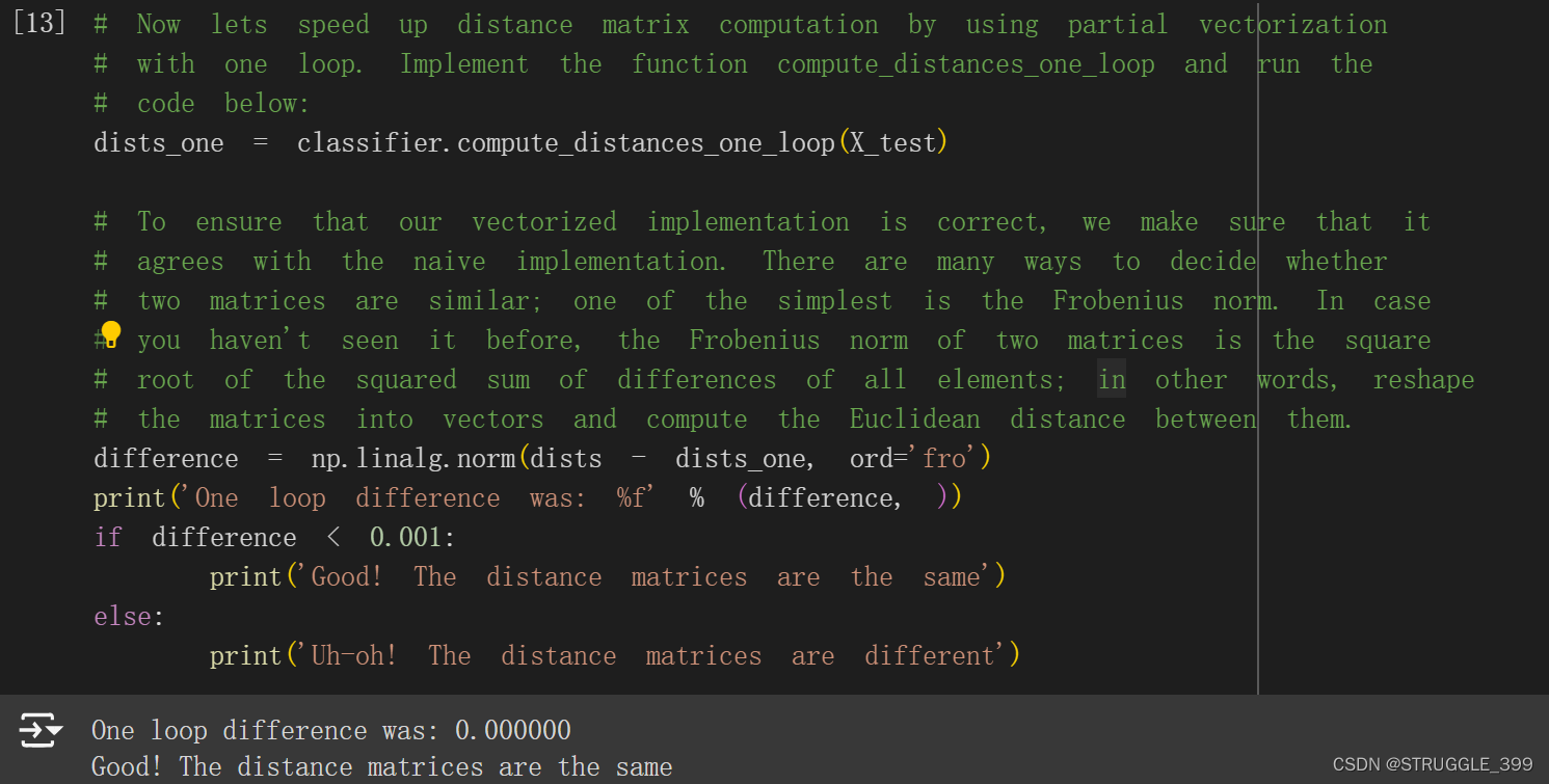
测试 compute_distances_one_loop 的实现,结果正确:
compute_distances_no_loops
不使用 for 循环,计算所有测试示例和所有训练示例之间的距离,首先我们将 L2 距离公式进行如下变形,将括号展开:
d
2
(
I
1
,
I
2
)
=
∑
p
(
I
1
p
−
I
2
p
)
2
=
∑
p
(
(
I
1
p
)
2
−
2
I
1
p
I
2
p
+
(
I
2
p
)
2
)
=
∑
p
(
I
1
p
)
2
−
2
∑
p
I
1
p
I
2
p
+
∑
p
(
I
2
p
)
2
\begin{aligned} d_2(I_1,I_2)&=\sqrt{\sum_p(I_1^p-I_2^p)^2}\\ &=\sqrt{\sum_p((I_1^p)^2-2I_1^pI_2^p+(I_2^p)^2)}\\ &=\sqrt{\sum_p(I_1^p)^2-2\sum_pI_1^pI_2^p+\sum_p(I_2^p)^2} \end{aligned}
d2(I1,I2)=p∑(I1p−I2p)2=p∑((I1p)2−2I1pI2p+(I2p)2)=p∑(I1p)2−2p∑I1pI2p+p∑(I2p)2
首先, dists[i, j] 表示第 i 个测试图片与第 j 个训练图片的 L2 距离。实现思路为:
- 通过表达式
np.square(X), axis=1, keepdims=True)计算 ∑ p ( I 1 p ) 2 \sum_p(I_1^p)^2 ∑p(I1p)2。 - 通过表达式
np.sum(np.square(self.X_train), axis=1))计算 ∑ p ( I 2 p ) 2 \sum_p(I_2^p)^2 ∑p(I2p)2。 - 通过表达式
np.dot(X, self.X_train.T)计算 ∑ p I 1 p I 2 p \sum_pI_1^pI_2^p ∑pI1pI2p。 - 将 1、2、3 组合起来,利用广播机制计算
dists。
【注意】计算
∑
p
(
I
1
p
)
2
\sum_p(I_1^p)^2
∑p(I1p)2 时使用了带有 keepdims=True 参数的 np.sum 函数,目的是在计算 dists 时让其按列广播,具体原因与 dists 定义相关。
def compute_distances_no_loops(self, X):
    """
    Compute the distance between each test point in X and each training point
    in self.X_train using no explicit loops.

    Input / Output: Same as compute_distances_two_loops
    """
    num_test = X.shape[0]
    num_train = self.X_train.shape[0]
    dists = np.zeros((num_test, num_train))
    #########################################################################
    # TODO:                                                                 #
    # Compute the l2 distance between all test points and all training      #
    # points without using any explicit loops, and store the result in      #
    # dists.                                                                #
    #                                                                       #
    # You should implement this function using only basic array operations; #
    # in particular you should not use functions from scipy,                #
    # nor use np.linalg.norm().                                             #
    #                                                                       #
    # HINT: Try to formulate the l2 distance using matrix multiplication    #
    #       and two broadcast sums.                                         #
    #########################################################################
    # *****START OF YOUR CODE (DO NOT DELETE/MODIFY THIS LINE)*****

    dists = np.sqrt(np.sum(np.square(X), axis=1, keepdims=True)
                    - 2 * np.dot(X, self.X_train.T)
                    + np.sum(np.square(self.X_train), axis=1))

    # *****END OF YOUR CODE (DO NOT DELETE/MODIFY THIS LINE)*****
    return dists
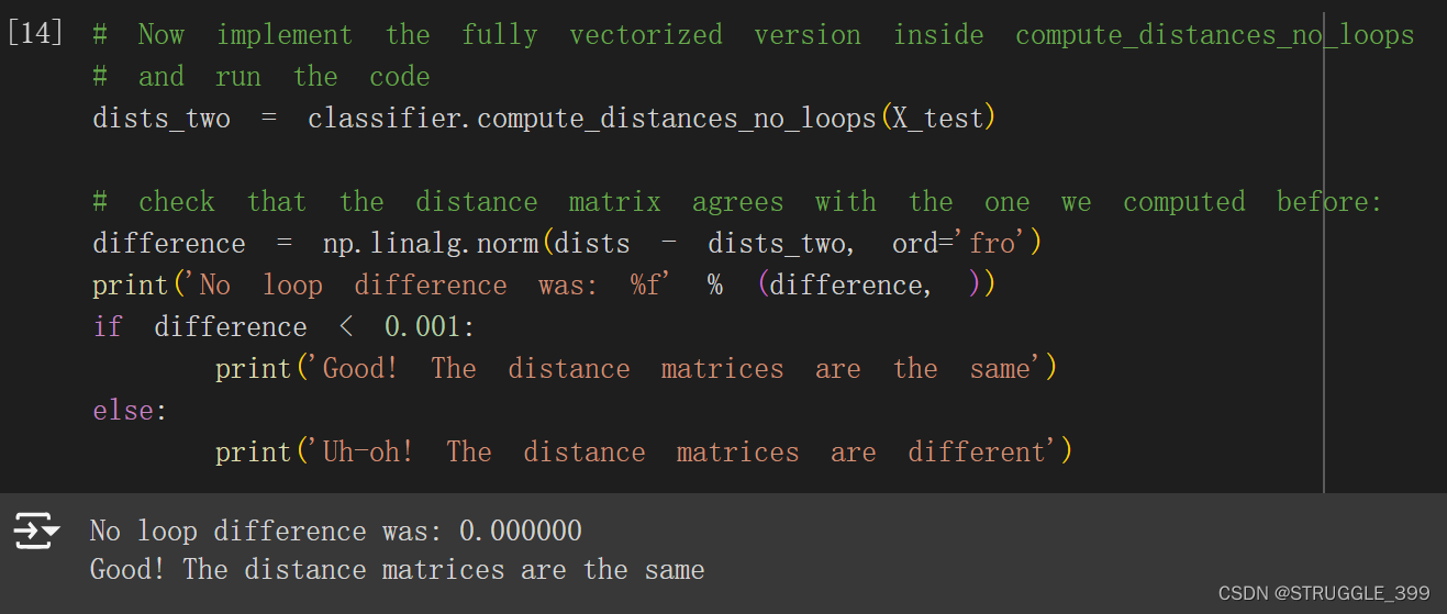
测试 compute_distances_no_loops 的实现,结果正确:
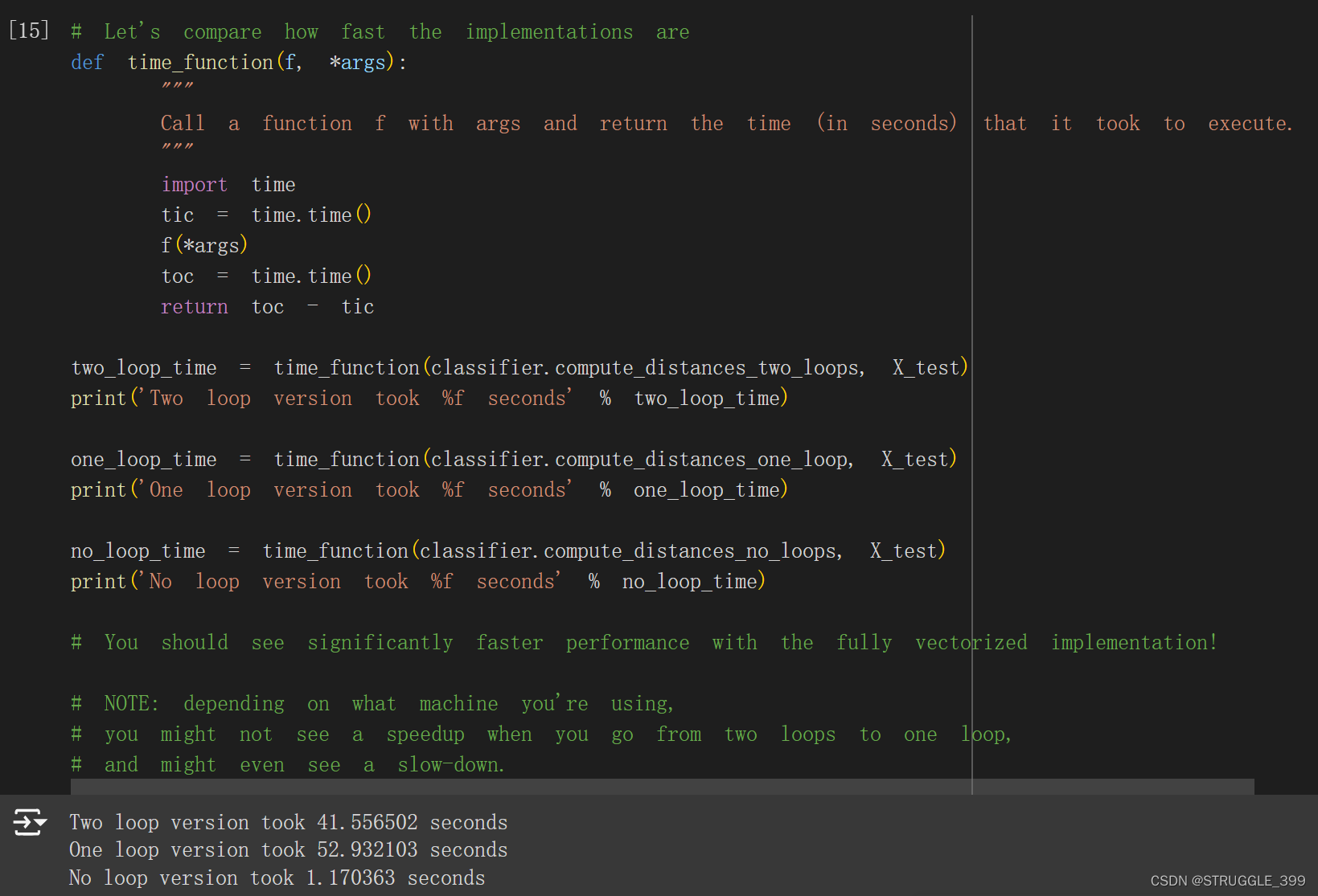
最后,我们比较三个版本的距离计算时间,可以看到,不使用循环的版本(全向量化代码实现)快很多!
Cross Validation
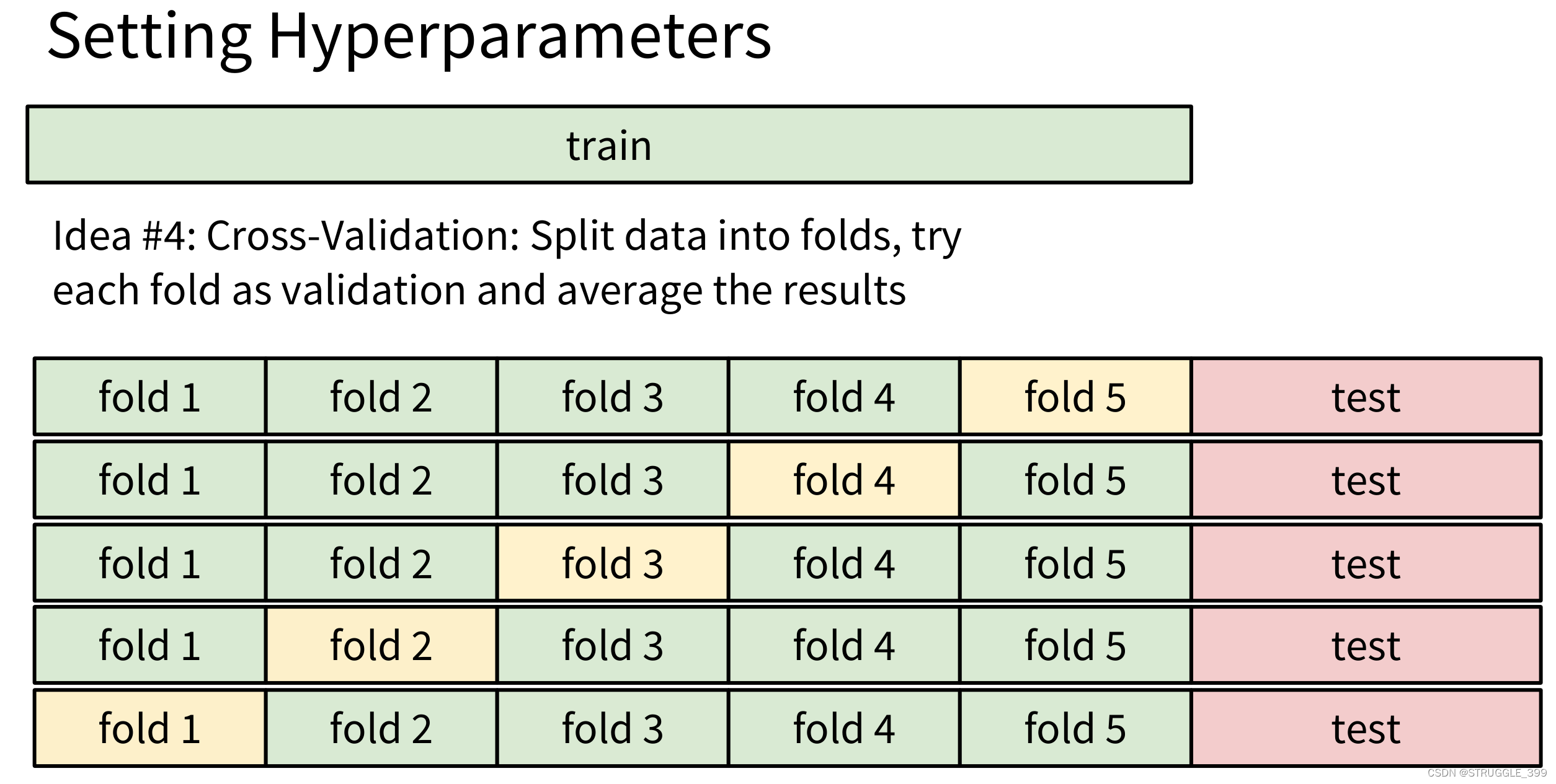
K 折交叉验证的思想如下图所示(图示为 5 折交叉验证):
- 将训练数据分为
num_folds份。 - 将每一份作为验证集,剩余部分作为训练集,计算验证精度。
- 计算平均验证精度。
使用交叉验证进行超参数调整(Hyper parameter tuning)的步骤为:
- 通过
numpy.array_split函数将训练数据分为num_folds份。 - 遍历每一组超参数,将每一份作为验证集,剩余部分作为训练集,计算验证精度,进而计算平均验证精度。
- 选择平均验证精度最高对应的那一组超参数作为调参的结果。
num_folds = 5
k_choices = [1, 3, 5, 8, 10, 12, 15, 20, 50, 100]

X_train_folds = []
y_train_folds = []
################################################################################
# TODO:                                                                        #
# Split up the training data into folds. After splitting, X_train_folds and    #
# y_train_folds should each be lists of length num_folds, where                #
# y_train_folds[i] is the label vector for the points in X_train_folds[i].     #
# Hint: Look up the numpy array_split function.                                #
################################################################################
# *****START OF YOUR CODE (DO NOT DELETE/MODIFY THIS LINE)*****

# 将训练集等分为 num_folds 份
X_train_folds = np.array_split(X_train, num_folds)
y_train_folds = np.array_split(y_train, num_folds)

# *****END OF YOUR CODE (DO NOT DELETE/MODIFY THIS LINE)*****

# A dictionary holding the accuracies for different values of k that we find
# when running cross-validation. After running cross-validation,
# k_to_accuracies[k] should be a list of length num_folds giving the different
# accuracy values that we found when using that value of k.
k_to_accuracies = {}


################################################################################
# TODO:                                                                        #
# Perform k-fold cross validation to find the best value of k. For each        #
# possible value of k, run the k-nearest-neighbor algorithm num_folds times,   #
# where in each case you use all but one of the folds as training data and the #
# last fold as a validation set. Store the accuracies for all fold and all     #
# values of k in the k_to_accuracies dictionary.                               #
################################################################################
# *****START OF YOUR CODE (DO NOT DELETE/MODIFY THIS LINE)*****

for k in k_choices:
  k_to_accuracies[k] = []
  for m in range(num_folds):
    # 使用第 m fold 作为 validation fold.
    knn = KNearestNeighbor()
    # 划分训练集和验证集
    X_train_set = np.concatenate(X_train_folds[:m] + X_train_folds[m+1:])
    y_train_set = np.concatenate(y_train_folds[:m] + y_train_folds[m+1:])
    X_validation_set = X_train_folds[m]
    y_validation_set = y_train_folds[m]

    knn.train(X_train_set, y_train_set)
    Y_preds = knn.predict(X_validation_set, k=k) # 获取预测结果
    acc = np.mean(Y_preds == y_validation_set) # 计算预测正确率
    k_to_accuracies[k].append(acc)

# *****END OF YOUR CODE (DO NOT DELETE/MODIFY THIS LINE)*****

# Print out the computed accuracies
for k in sorted(k_to_accuracies):
    for accuracy in k_to_accuracies[k]:
        print('k = %d, accuracy = %f' % (k, accuracy))
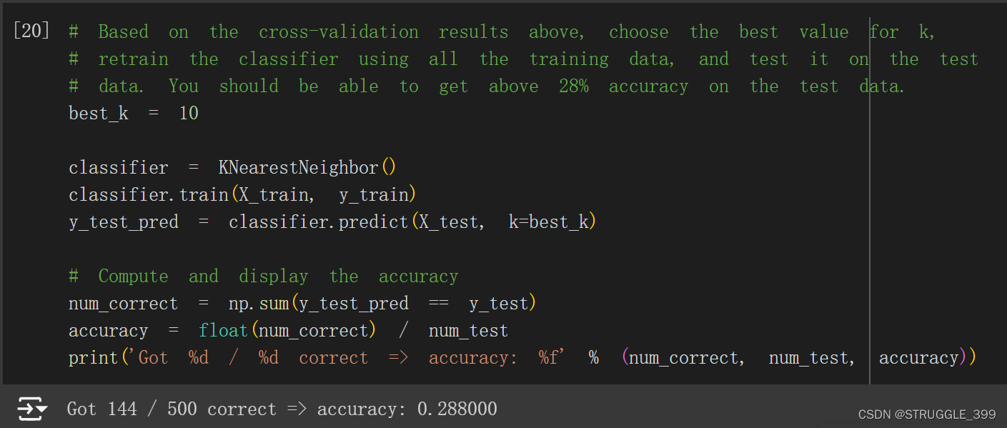
最终的结果如下图所示,折线表示平均精度,由此可见 k=10 时平均验证精度最高,因此 best_k=10。
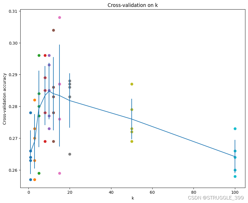
最终,我们设置 k=10,进行测试,得到测试精度为 28.8%,与题中描述一致。
Inline Question 3:
在分类设置中,对于所有 k,以下哪些关于 k -Nearest Neighbor ( k -NN) 的说法是正确的?选择所有适用的。
- k-NN 分类器的决策边界是线性的。
- 1-NN 的训练误差总是低于或等于 5-NN 的误差。
- 1-NN 的测试误差总是低于 5-NN 的测试误差。
- 使用 k-NN 分类器对测试示例进行分类所需的时间随训练集的大小而增长。
- 以上都不是。
【答】2、4,解释如下:
- k-NN 分类器的决策边界是非线性的。
- 1-NN 的训练误差始终为零,因为与其最近的图片就是其本身,因此训练误差为零,5-NN 的训练误差则不一定为零。
- 不一定,5-NN 的测试误差可能更低。
- k-NN 分类器在预测时,需要计算预测图片与所有训练图片的距离,因此分类时间随着训练集大小而增长。
Q2: Training a Support Vector Machine
SVM 分类器是线性分类器,为每一张测试图片计算一个得分向量,得分最高的类别即为 SVM 分类器预测的结果,得分向量的计算公式如下:
s
=
f
(
x
,
W
,
b
)
=
W
x
+
b
s=f(x,W,b)=Wx+b
s=f(x,W,b)=Wx+b
其中,
W
W
W 和
b
b
b 为参数。SVM 分类器的损失函数(loss function)为:
L
i
=
∑
j
≠
y
i
max
(
0
,
s
j
−
s
y
i
+
Δ
)
L_i=\sum_{j\ne y_i}\max(0,s_j-s_{y_i}+\Delta)
Li=j=yi∑max(0,sj−syi+Δ)
其中,
Δ
\Delta
Δ 为超参数,在该作业中
Δ
=
1
\Delta=1
Δ=1。SVM 分类器的代价函数(cost function)为:
L
=
1
N
∑
i
∑
j
≠
y
i
max
(
0
,
s
j
−
s
y
i
+
Δ
)
⏟
data loss
+
1
2
λ
∑
k
∑
l
W
k
,
l
2
⏟
regularization loss
L=\underbrace{\frac{1}{N}\sum_i\sum_{j\ne y_i}\max(0,s_j-s_{y_i}+\Delta)}_{\text{data loss}}+ \underbrace{\frac{1}{2}\lambda\sum_k\sum_lW_{k,l}^2}_{\text{regularization loss}}
L=data loss
N1i∑j=yi∑max(0,sj−syi+Δ)+regularization loss
21λk∑l∑Wk,l2
其中,
λ
\lambda
λ(正则化强度)为超参数,前面乘以 0.5 是因为在计算梯度时可以将其消除,无需在前面乘以梯度。
svm_loss_naive
可参考 cs231n 课程笔记中的 SVM 损失函数的实现代码,其中包含完全非向量化的实现和半向量化的实现。
使用两个 for 循环,计算 SVM 损失,实现思路为:
- 遍历每一张训练图片,计算对应的得分向量
scores,正确类别对应的得分correct_class_score = scores[y[i]]。 - 遍历每个类别的得分(正确类别得分除外),loss 累加上
margin = max(0, scores[j] - correct_class_score + 1)。 - 当
magin > 0时,出现非零项,需要更新dW,dW的第 j 列加上X[i].T,第y[i]列减去X[i].T。
def svm_loss_naive(W, X, y, reg):
    """
    Structured SVM loss function, naive implementation (with loops).

    Inputs have dimension D, there are C classes, and we operate on minibatches
    of N examples.

    Inputs:
    - W: A numpy array of shape (D, C) containing weights.
    - X: A numpy array of shape (N, D) containing a minibatch of data.
    - y: A numpy array of shape (N,) containing training labels; y[i] = c means
      that X[i] has label c, where 0 <= c < C.
    - reg: (float) regularization strength

    Returns a tuple of:
    - loss as single float
    - gradient with respect to weights W; an array of same shape as W
    """
    dW = np.zeros(W.shape)  # initialize the gradient as zero

    # compute the loss and the gradient
    num_classes = W.shape[1]
    num_train = X.shape[0]
    loss = 0.0
    #############################################################################
    # TODO:                                                                     #
    # Implement a unvectorized version of the structured SVM loss, storing the    #
    # result in loss.                                                           #
    #############################################################################
    # *****START OF YOUR CODE (DO NOT DELETE/MODIFY THIS LINE)*****

    for i in range(num_train):
        scores = X[i].dot(W)
        correct_class_score = scores[y[i]]
        for j in range(num_classes):
            if j == y[i]:
              continue
            margin = max(0, scores[j] - correct_class_score + 1)  # note delta = 1
            loss += margin
            if margin > 0:
              # 出现非零项, 与矩阵W的第j列和第y[i]列相关
              dW[:, j] += X[i]
              dW[:, y[i]] -= X[i]

    # *****END OF YOUR CODE (DO NOT DELETE/MODIFY THIS LINE)*****

    # Right now the loss is a sum over all training examples, but we want it
    # to be an average instead so we divide by num_train.
    loss /= num_train
    dW /= num_train
    # Add regularization to the loss.
    loss += 0.5 * reg * np.sum(np.square(W))

    #############################################################################
    # TODO:                                                                     #
    # Compute the gradient of the loss function and store it dW.                #
    # Rather that first computing the loss and then computing the derivative,   #
    # it may be simpler to compute the derivative at the same time that the     #
    # loss is being computed. As a result you may need to modify some of the    #
    # code above to compute the gradient.                                       #
    #############################################################################
    # *****START OF YOUR CODE (DO NOT DELETE/MODIFY THIS LINE)*****

    # data loss的导数 + regularization loss 的导数就是 dW
    dW += reg * W

    # *****END OF YOUR CODE (DO NOT DELETE/MODIFY THIS LINE)*****

    return loss, dW
【注意】上面的代码实现中没有涉及到参数 b,是因为进行了预处理操作,在图片向量添加了一个维度,其值固定为1,而参数矩阵 W 也增加一个维度,这一维就是原始的参数 b。
梯度推导
SVM 代价函数(cost function)为:
L
=
1
N
∑
i
∑
j
≠
y
i
max
(
0
,
f
(
x
i
;
W
)
j
−
f
(
x
i
;
W
)
y
i
+
Δ
)
⏟
data loss
+
1
2
λ
∑
k
∑
l
W
k
,
l
2
⏟
regularization loss
L=\underbrace{\frac{1}{N}\sum_i\sum_{j\ne y_i}\max(0,f(x_i;W)_j-f(x_i;W)_{y_i}+\Delta)}_{\text{data loss}}+ \underbrace{\frac{1}{2}\lambda\sum_k\sum_lW_{k,l}^2}_{\text{regularization loss}}
L=data loss
N1i∑j=yi∑max(0,f(xi;W)j−f(xi;W)yi+Δ)+regularization loss
21λk∑l∑Wk,l2 由于:
f
(
x
i
;
W
)
j
=
x
i
1
w
1
j
+
x
i
2
w
2
j
+
⋯
+
x
i
D
w
D
j
f(x_i;W)_j=x_{i1}w_{1j}+x_{i2}w_{2j}+\cdots+x_{iD}w_{Dj}
f(xi;W)j=xi1w1j+xi2w2j+⋯+xiDwDj 因此,
f
(
x
i
;
W
)
j
f(x_i;W)_j
f(xi;W)j 与参数矩阵 W 的第 j 列有关:
∂
∂
w
k
j
f
(
x
i
;
W
)
j
=
x
i
k
,
(
1
≤
k
≤
D
)
\frac{\partial }{\partial w_{kj}}f(x_i;W)_j = x_{ik},(1\le k \le D)
∂wkj∂f(xi;W)j=xik,(1≤k≤D) 同理,
f
(
x
i
;
W
)
y
i
f(x_i;W)_{y_i}
f(xi;W)yi 与参数矩阵 W 的第 yi 列有关,因此,在 margin = max(0, scores[j] - correct_class_score + 1) 大于 0 的情况下,需要更新 dW 的第 j 列和第 yi 列,分别加上
x
i
T
x_i^T
xiT、
−
x
i
T
-x_i^T
−xiT(其中
x
i
x_i
xi 为第 i 个训练图片向量(行向量))。
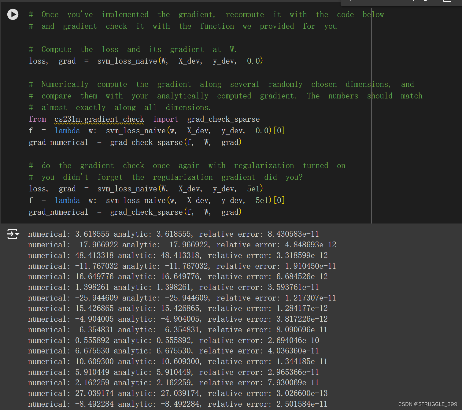
运行梯度检查,测试结果如下,误差几乎为零,测试通过:
svm_loss_half_vectorized
在实现全向量化实现前,先完成半向量化(仅使用一个 for 循环)的实现,实现的思路为:
- 遍历每一个训练图片,计算得分向量
scores,正确类别对应的得分correct_class_score = scores[y[i]]。。 - 通过
np.maximum(0, scores - correct_class_score + 1)计算margins向量,margins的每个分量之和就是该训练图片的损失(注意需要margins[y[i]] = 0)。 - 将
margins向量中每个大于 0 的分量置为 1(因为dW与 margins 的具体值无关,只要大于0即可)。 - 将正确分类对应的
margins分量置为margins向量大于 0 的分量个数的相反数。 dW累加上np.dot(X[i].reshape(-1, 1), margins)。
【注】该半向量化实现不是作业要求的,只是为了更平滑地过渡到全向量化代码的实现。前两步为损失计算,后三步为梯度计算。
def svm_loss_half_vectorized(W, X, y, reg):
    """
    Structured SVM loss function, vectorized implementation.

    Inputs and outputs are the same as svm_loss_naive.
    """
    loss = 0.0
    dW = np.zeros(W.shape)  # initialize the gradient as zero
    num_train = X.shape[0]
    num_classes = W.shape[1]

    for i in range(num_train):
        scores = X[i].dot(W)
        correct_class_score = scores[y[i]]
        margins = np.maximum(0, scores - correct_class_score + 1) # delta = 1
        margins[y[i]] = 0
        loss += np.sum(margins)

        margins[margins > 0] = 1
        margins[y[i]] = -np.sum(margins)
        dW += np.dot(X[i].reshape(-1, 1), margins)


    loss /= num_train
    dW /= num_train

    # 加上正则化项的损失和梯度
    loss += 0.5 * reg * np.sum(np.square(W))
    dW += reg * W

    return loss, dW
由 svm_loss_naive 分析可知,当 margins[j] > 0 时, 矩阵 dW 的第 j 列和第 yi 列分别需要加上
x
i
T
x_i^T
xiT、
−
x
i
T
-x_i^T
−xiT,将 margins 进行第4、5 步的处理后,
x
i
T
x_i^T
xiT (列向量)与 margins(行向量)作矩阵乘法,得到的矩阵具有如下性质:
- 若
margins[j] > 0,则得到的矩阵第 j 列为 x i T x_i^T xiT。 - 矩阵第 yi 列为
-num倍的 x i T x_i^T xiT,其中num为margins向量中分量大于零的个数。
将此矩阵加到 dW 即可完成一个训练图片的损失计算。
svm_loss_vectorized
有了半向量化实现的思路,只需要做一些调整即可,不使用循环的实现的思路为:
- 通过
X.dot(W)(矩阵乘法), 计算得分矩阵scores,获取每个训练图片正确分类类别的得分,存放于列表correct_class_scores中。 - 通过
np.maximum(0, scores - correct_class_scores + 1)计算margins矩阵,margins的每个分量之和就是所有训练图片的损失(注意需要margins[range(num_train), y] = 0)。 - 将
margins向量中每个大于 0 的分量置为 1。 - 将正确分类对应的
margins分量置为margins向量大于 0 的分量个数的相反数。 dW累加上np.dot(X.T, margins)。
def svm_loss_vectorized(W, X, y, reg):
    """
    Structured SVM loss function, vectorized implementation.

    Inputs and outputs are the same as svm_loss_naive.
    """
    loss = 0.0
    dW = np.zeros(W.shape)  # initialize the gradient as zero

    #############################################################################
    # TODO:                                                                     #
    # Implement a vectorized version of the structured SVM loss, storing the    #
    # result in loss.                                                           #
    #############################################################################
    # *****START OF YOUR CODE (DO NOT DELETE/MODIFY THIS LINE)*****

    num_train = X.shape[0]
    num_classes = W.shape[1]
    scores = np.dot(X, W)
    # 获取每个 x 正确分类类别的得分
    correct_class_scores = scores[range(num_train), y].reshape(-1, 1)
    margins = np.maximum(0, scores - correct_class_scores + 1)
    # 将正确分类的margins置为0
    margins[range(num_train), y] = 0
    loss += np.sum(margins) / num_train
    loss += 0.5 * reg * np.sum(np.square(W))

    # *****END OF YOUR CODE (DO NOT DELETE/MODIFY THIS LINE)*****

    #############################################################################
    # TODO:                                                                     #
    # Implement a vectorized version of the gradient for the structured SVM     #
    # loss, storing the result in dW.                                           #
    #                                                                           #
    # Hint: Instead of computing the gradient from scratch, it may be easier    #
    # to reuse some of the intermediate values that you used to compute the     #
    # loss.                                                                     #
    #############################################################################
    # *****START OF YOUR CODE (DO NOT DELETE/MODIFY THIS LINE)*****
    margins[margins > 0] = 1
    margins[range(num_train),y] = -np.sum(margins, axis=1)
    dW += np.dot(X.T, margins) / num_train + reg * W

    # *****END OF YOUR CODE (DO NOT DELETE/MODIFY THIS LINE)*****
    return loss, dW
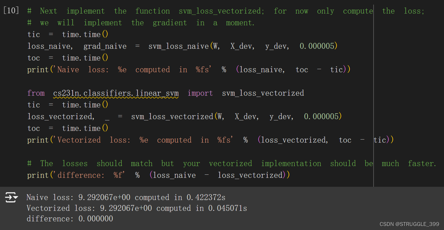
进行损失的测试,损失与 svm_loss_naive 的差异为零,测试通过:
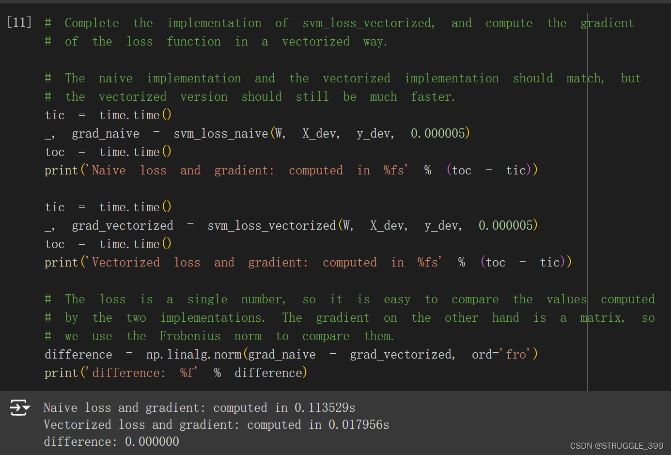
进行梯度的测试,梯度与 svm_loss_naive 的差异为零,测试通过:
Stochastic Gradient Descent (SGD)
我们现在已经有了向量化的 SVM 损失实现,我们可以使用 SGD 最小化 SVM 代价函数。具体实现中,我们使用的是小批量随机梯度下降(minibatch SGD),实现的思路为:
- 随机选择一部分训练样本(样本大小为
batch_size),通过np.random.choice(num_train, size=batch_size)可随机生成[0, num_train-1]之间的整数下标列表(长度为batch_size)。 - 根据这部分样本,计算 SVM 损失和梯度。
- 运行梯度下降,进行参数 W 的更新。
def train(
        self,
        X,
        y,
        learning_rate=1e-3,
        reg=1e-5,
        num_iters=100,
        batch_size=200,
        verbose=False,
    ):
    """
    Train this linear classifier using stochastic gradient descent.

    Inputs:
    - X: A numpy array of shape (N, D) containing training data; there are N
      training samples each of dimension D.
    - y: A numpy array of shape (N,) containing training labels; y[i] = c
      means that X[i] has label 0 <= c < C for C classes.
    - learning_rate: (float) learning rate for optimization.
    - reg: (float) regularization strength.
    - num_iters: (integer) number of steps to take when optimizing
    - batch_size: (integer) number of training examples to use at each step.
    - verbose: (boolean) If true, print progress during optimization.

    Outputs:
    A list containing the value of the loss function at each training iteration.
    """
    num_train, dim = X.shape
    num_classes = (
        np.max(y) + 1
    )  # assume y takes values 0...K-1 where K is number of classes
    if self.W is None:
        # lazily initialize W
        self.W = 0.001 * np.random.randn(dim, num_classes)

    # Run stochastic gradient descent to optimize W
    loss_history = []
    for it in range(num_iters):
        X_batch = None
        y_batch = None

        #########################################################################
        # TODO:                                                                 #
        # Sample batch_size elements from the training data and their           #
        # corresponding labels to use in this round of gradient descent.        #
        # Store the data in X_batch and their corresponding labels in           #
        # y_batch; after sampling X_batch should have shape (batch_size, dim)   #
        # and y_batch should have shape (batch_size,)                           #
        #                                                                       #
        # Hint: Use np.random.choice to generate indices. Sampling with         #
        # replacement is faster than sampling without replacement.              #
        #########################################################################
        # *****START OF YOUR CODE (DO NOT DELETE/MODIFY THIS LINE)*****

        idxs = np.random.choice(num_train, size=batch_size)
        X_batch, y_batch = X[idxs], y[idxs]

        # *****END OF YOUR CODE (DO NOT DELETE/MODIFY THIS LINE)*****

        # evaluate loss and gradient
        loss, grad = self.loss(X_batch, y_batch, reg)
        loss_history.append(loss)

        # perform parameter update
        #########################################################################
        # TODO:                                                                 #
        # Update the weights using the gradient and the learning rate.          #
        #########################################################################
        # *****START OF YOUR CODE (DO NOT DELETE/MODIFY THIS LINE)*****

        self.W = self.W - learning_rate * grad

        # *****END OF YOUR CODE (DO NOT DELETE/MODIFY THIS LINE)*****

        if verbose and it % 100 == 0:
            print("iteration %d / %d: loss %f" % (it, num_iters, loss))

    return loss_history
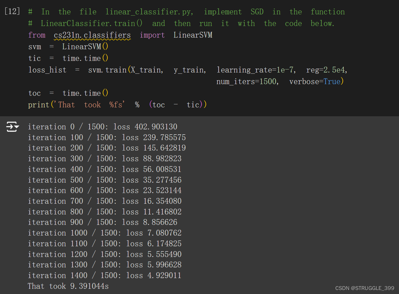
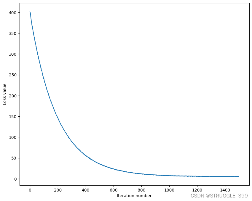
运行测试,SGD 的每一次迭代,SVM 的损失呈下降趋势,算法正确:
损失随迭代次数的变化如下图所示:
线性分类器的预测函数特别简单,实现思路如下:
- 计算得分矩阵
scores。 - 预测类别就是得分向量中分量最大的下标,通过
numpy.argmax实现。
def predict(self, X):
    """
    Use the trained weights of this linear classifier to predict labels for
    data points.

    Inputs:
    - X: A numpy array of shape (N, D) containing training data; there are N
      training samples each of dimension D.

    Returns:
    - y_pred: Predicted labels for the data in X. y_pred is a 1-dimensional
      array of length N, and each element is an integer giving the predicted
      class.
    """
    y_pred = np.zeros(X.shape[0])
    ###########################################################################
    # TODO:                                                                   #
    # Implement this method. Store the predicted labels in y_pred.            #
    ###########################################################################
    # *****START OF YOUR CODE (DO NOT DELETE/MODIFY THIS LINE)*****

    scores = np.dot(X, self.W) # 计算得分
    y_pred = np.argmax(scores, axis=1)

    # *****END OF YOUR CODE (DO NOT DELETE/MODIFY THIS LINE)*****
    return y_pred
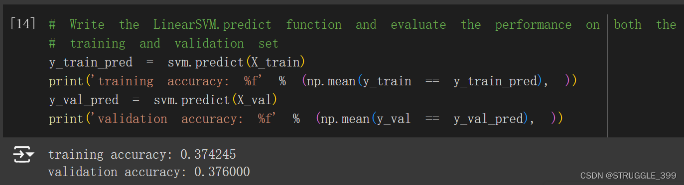
运行测试,可得训练精度和验证精度:
接下来进行超参数调整(Hyperparameter tuning),修改原始的 learning_rates 和 regularization_strengths 列表,增加更多的超参数以供搜索。实现的思路如下:
- 遍历每一组超参数,在该超参数设定下进行 SVM 的训练。
- 进行预测,计算训练精度、验证精度。
- 记录最佳验证精度,以及对应的 SVM 分类器。
# Use the validation set to tune hyperparameters (regularization strength and
# learning rate). You should experiment with different ranges for the learning
# rates and regularization strengths; if you are careful you should be able to
# get a classification accuracy of about 0.39 (> 0.385) on the validation set.
# Note: you may see runtime/overflow warnings during hyper-parameter search.
# This may be caused by extreme values, and is not a bug.
# results is dictionary mapping tuples of the form
# (learning_rate, regularization_strength) to tuples of the form
# (training_accuracy, validation_accuracy). The accuracy is simply the fraction
# of data points that are correctly classified.
results = {}
best_val = -1 # The highest validation accuracy that we have seen so far.
best_svm = None # The LinearSVM object that achieved the highest validation rate.
################################################################################
# TODO: #
# Write code that chooses the best hyperparameters by tuning on the validation #
# set. For each combination of hyperparameters, train a linear SVM on the #
# training set, compute its accuracy on the training and validation sets, and #
# store these numbers in the results dictionary. In addition, store the best #
# validation accuracy in best_val and the LinearSVM object that achieves this #
# accuracy in best_svm. #
# #
# Hint: You should use a small value for num_iters as you develop your #
# validation code so that the SVMs don't take much time to train; once you are #
# confident that your validation code works, you should rerun the validation #
# code with a larger value for num_iters. #
################################################################################
# Provided as a reference. You may or may not want to change these hyperparameters
learning_rates = [1e-7, 3e-7, 1e-6, 3e-6, 1e-5, 3e-5, 1e-4, 3e-4, 1e-3, 3e-3, 1e-2, 3e-2]
regularization_strengths = [1e4, 1.5e4, 2e4, 2.5e4, 3e4, 3.5e4, 4e4, 4.5e4, 5e4]
# *****START OF YOUR CODE (DO NOT DELETE/MODIFY THIS LINE)*****
for lr in learning_rates:
for reg in regularization_strengths:
svm = LinearSVM()
loss_hist = svm.train(X_train, y_train, learning_rate=lr, reg=reg,
num_iters=500, verbose=True)
y_train_pred = svm.predict(X_train)
y_val_pred = svm.predict(X_val)
training_accuracy = np.mean(y_train == y_train_pred)
validation_accuracy = np.mean(y_val == y_val_pred)
results[(lr, reg)] = (training_accuracy, validation_accuracy)
if best_val < validation_accuracy:
best_val = validation_accuracy
best_svm = svm
# *****END OF YOUR CODE (DO NOT DELETE/MODIFY THIS LINE)*****
# Print out results.
for lr, reg in sorted(results):
train_accuracy, val_accuracy = results[(lr, reg)]
print('lr %e reg %e train accuracy: %f val accuracy: %f' % (
lr, reg, train_accuracy, val_accuracy))
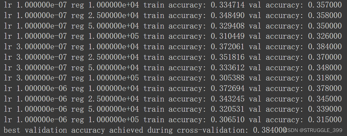
print('best validation accuracy achieved during cross-validation: %f' % best_val)
结果如下图所示:
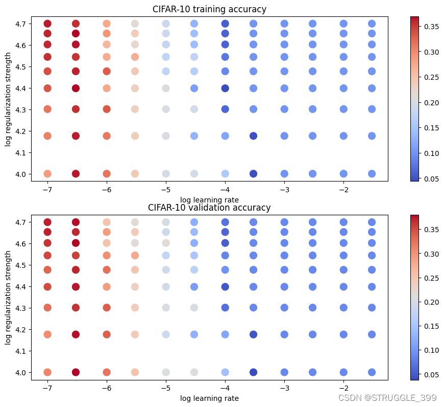
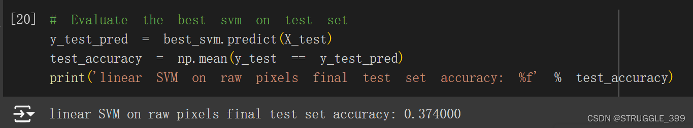
利用 best_svm 进行预测,测试精度为 37.4%。
最后,将 SVM 学习到的权重参数 W 进行可视化:
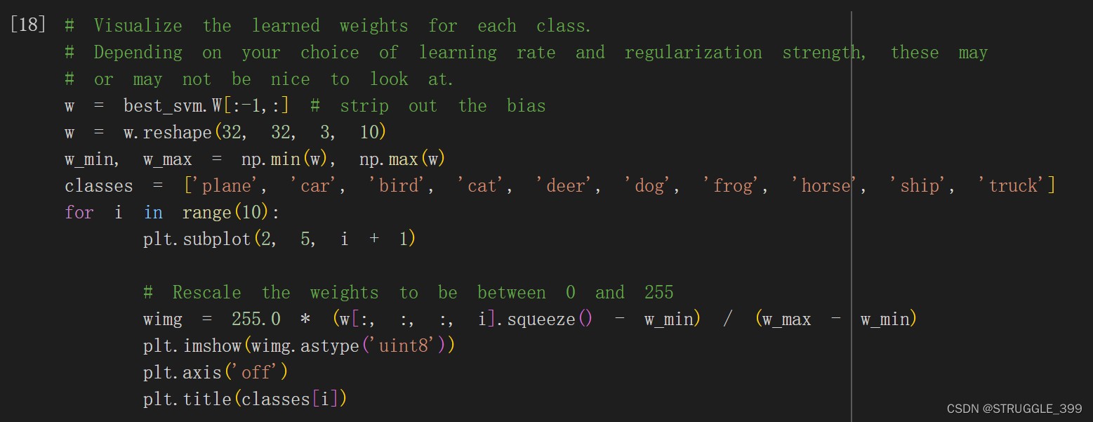
可视化结果如下:
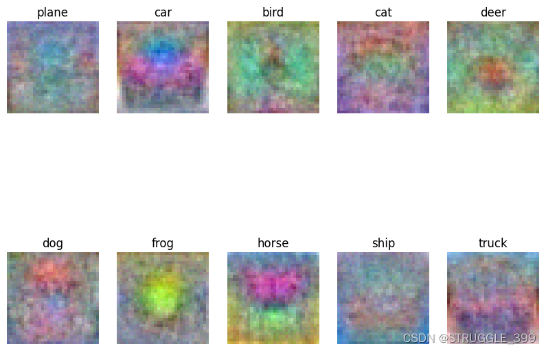
Inline Question 2
描述可视化 SVM 权重的外观,并简要解释其外观的原因。
【答】SVM 权重的外观与对应类别的图片形状相似,比较明显的类别是 car、frog、horse 等。出现这种外观的原因是因为 SVM 分类器实质上是在做模板匹配,SVM 分类器在训练时会为每一个类别的图片学习一个模板,这个模板会平均同一类别的所有图片的差异。
Q3: Implement a Softmax classifier
Softmax 分类器也是一个线性分类器,与 SVM 分类器的区别是其损失函数不同,Softmax 的损失函数为交叉熵函数(cross entropy function):
L
i
=
−
log
(
e
f
y
i
∑
j
e
f
j
)
=
log
(
∑
j
e
f
j
)
−
f
y
i
L_i=-\log(\frac{e^{f_{y_i}}}{\sum_j e^{f_j}})=\log(\sum_j e^{f_j})-f_{y_i}
Li=−log(∑jefjefyi)=log(j∑efj)−fyi
Softmax 分类器的代价函数为:
L
=
1
N
∑
i
[
log
(
∑
j
e
f
j
)
−
f
y
i
]
⏟
data loss
+
1
2
λ
∑
k
∑
l
W
k
,
l
2
⏟
regularization loss
L=\underbrace{\frac{1}{N}\sum_i [\log(\sum_j e^{f_j})-f_{y_i}]}_{\text{data loss}}+\underbrace{\frac{1}{2}\lambda\sum_k\sum_lW_{k,l}^2}_{\text{regularization loss}}
L=data loss
N1i∑[log(j∑efj)−fyi]+regularization loss
21λk∑l∑Wk,l2
损失函数梯度推导
∂
∂
w
k
l
L
i
=
{
e
f
l
∑
j
e
f
j
x
i
k
=
p
l
x
i
k
if
l
≠
y
i
e
f
l
∑
j
e
f
j
x
i
k
−
x
i
k
=
(
p
l
−
1
)
x
i
k
if
l
=
y
i
\frac{\partial}{\partial w_{kl}}L_i =\begin{cases} \frac{e^{f_{l}}}{\sum_j e^{f_j}}x_{ik}=p_{l}x_{ik} &\text{if } l\ne y_i\\ \frac{e^{f_{l}}}{\sum_j e^{f_j}}x_{ik}-x_{ik}=(p_{l}-1)x_{ik}&\text{if }l= y_i\\ \end{cases}
∂wkl∂Li=⎩
⎨
⎧∑jefjeflxik=plxik∑jefjeflxik−xik=(pl−1)xikif l=yiif l=yi
其中,
1
≤
k
≤
D
1\le k\le D
1≤k≤D,整理后可得:
∂
∂
w
k
l
L
i
=
{
p
l
x
i
k
if
l
≠
y
i
(
p
l
−
1
)
x
i
k
if
l
=
y
i
\frac{\partial}{\partial w_{kl}}L_i =\begin{cases} p_{l}x_{ik} &\text{if } l\ne y_i\\ (p_{l}-1)x_{ik}&\text{if }l= y_i\\ \end{cases}
∂wkl∂Li={plxik(pl−1)xikif l=yiif l=yi
softmax_loss_naive
梯度的推导过程如上所示,实现的思路为:
- 首先计算得分向量
score,然后将score的每一个分量减去最大分量值,保证数值稳定性(这一步不会影响损失和梯度)。 - 为了便于计算梯度,通过
p[y[i]] -= 1统一形式。 - 将
np.dot(X[i].reshape(-1, 1), p.reshape(1, -1))累加到dW。
def softmax_loss_naive(W, X, y, reg):
    """
    Softmax loss function, naive implementation (with loops)

    Inputs have dimension D, there are C classes, and we operate on minibatches
    of N examples.

    Inputs:
    - W: A numpy array of shape (D, C) containing weights.
    - X: A numpy array of shape (N, D) containing a minibatch of data.
    - y: A numpy array of shape (N,) containing training labels; y[i] = c means
      that X[i] has label c, where 0 <= c < C.
    - reg: (float) regularization strength

    Returns a tuple of:
    - loss as single float
    - gradient with respect to weights W; an array of same shape as W
    """
    # Initialize the loss and gradient to zero.
    loss = 0.0
    dW = np.zeros_like(W)

    #############################################################################
    # TODO: Compute the softmax loss and its gradient using explicit loops.     #
    # Store the loss in loss and the gradient in dW. If you are not careful     #
    # here, it is easy to run into numeric instability. Don't forget the        #
    # regularization!                                                           #
    #############################################################################
    # *****START OF YOUR CODE (DO NOT DELETE/MODIFY THIS LINE)*****

    num_train = X.shape[0]
    num_classes = W.shape[1]
    for i in range(num_train):
      score = X[i].dot(W)
      score -= max(score) # 防止溢出,保证数值稳定性
      p = np.exp(score) / np.sum(np.exp(score))
      loss += -np.log(p[y[i]])

      p[y[i]] -= 1 # 统一形式
      for j in range(num_classes):
        dW[:, j] += p[j] * X[i]


    loss /= num_train
    loss += 0.5 * reg * np.sum(np.square(W))
    dW /= num_train
    dW += reg * W
    # *****END OF YOUR CODE (DO NOT DELETE/MODIFY THIS LINE)*****

    return loss, dW
测试结果如下,与预期结果相近:
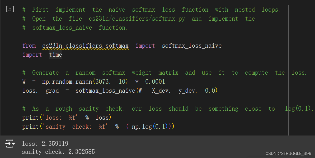
Inline Question 1
为什么我们预计损失接近-log(0.1)?请简要解释。
【答】因为我们随机产生参数 W,因而分类也是随机的,CIFAR-10 共有 10 个类别的图片,因此分类正确的概率为 10%,所以 softmax loss 应该接近 -log(0.1)。
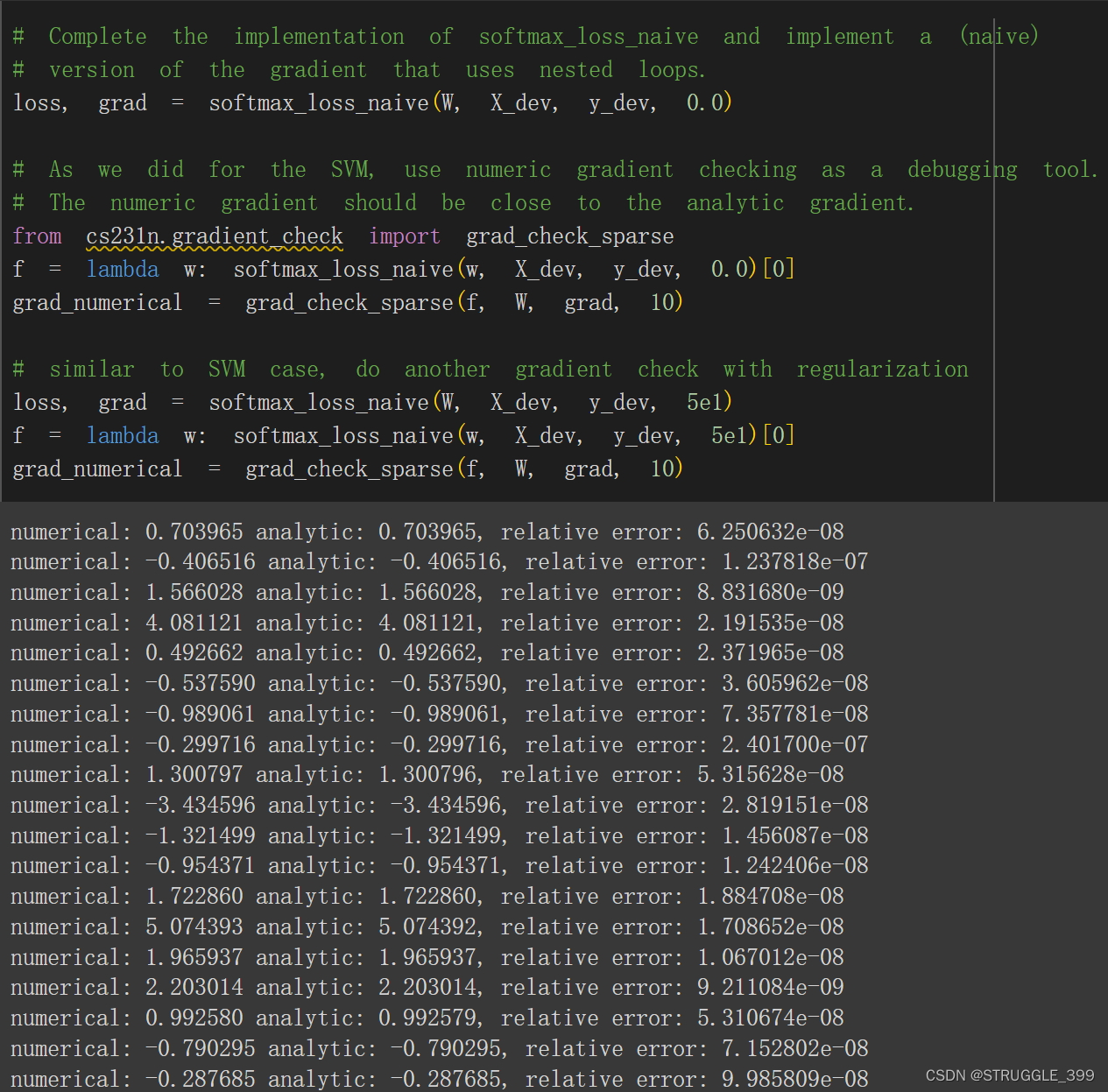
梯度测试如下,解析梯度和数值梯度相差几乎为零,梯度测试通过:
softmax_loss_half_vectorized
该实现为半向量化实现,作业中没有要求此实现,实际上就是使用一个 for 循环计算损失和梯度,主要是为了更好地过渡到全向量化代码的实现。
softmax_loss_naive 内层循环是很容易优化的,只需要计算
x
i
T
x_i^T
xiT 与 p 的乘积(矩阵乘法),加到 dW 即可。
def softmax_loss_half_vectorized(W, X, y, reg):
    """
    Softmax loss function, naive implementation (with loops)

    Inputs have dimension D, there are C classes, and we operate on minibatches
    of N examples.

    Inputs:
    - W: A numpy array of shape (D, C) containing weights.
    - X: A numpy array of shape (N, D) containing a minibatch of data.
    - y: A numpy array of shape (N,) containing training labels; y[i] = c means
      that X[i] has label c, where 0 <= c < C.
    - reg: (float) regularization strength

    Returns a tuple of:
    - loss as single float
    - gradient with respect to weights W; an array of same shape as W
    """
    # Initialize the loss and gradient to zero.
    loss = 0.0
    dW = np.zeros_like(W)

    #############################################################################
    # TODO: Compute the softmax loss and its gradient using explicit loops.     #
    # Store the loss in loss and the gradient in dW. If you are not careful     #
    # here, it is easy to run into numeric instability. Don't forget the        #
    # regularization!                                                           #
    #############################################################################
    # *****START OF YOUR CODE (DO NOT DELETE/MODIFY THIS LINE)*****

    num_train = X.shape[0]
    num_classes = W.shape[1]
    for i in range(num_train):
      score = X[i].dot(W)
      score -= max(score) # 防止溢出,保证数值稳定性
      p = np.exp(score) / np.sum(np.exp(score))
      loss += -np.log(p[y[i]])

      p[y[i]] -= 1
      dW += np.dot(X[i].reshape(-1, 1), p.reshape(1, -1))


    loss /= num_train
    loss += 0.5 * reg * np.sum(np.square(W))
    dW /= num_train
    dW += reg * W

    # *****END OF YOUR CODE (DO NOT DELETE/MODIFY THIS LINE)*****

    return loss, dW
softmax_loss_vectorized
完成半向量化实现后,做一些调整即可完成全向量化实现,实现思路如下:
- 计算得分矩阵
scores,将scores做与softmax_loss_naive相同的处理,以保证数值稳定性(这一步不会影响损失和梯度)。 - 计算概率矩阵
p。 - 剩下的损失、梯度计算与
softmax_loss_half_vectorized类似。
def softmax_loss_vectorized(W, X, y, reg):
    """
    Softmax loss function, vectorized version.

    Inputs and outputs are the same as softmax_loss_naive.
    """
    # Initialize the loss and gradient to zero.
    loss = 0.0
    dW = np.zeros_like(W)

    #############################################################################
    # TODO: Compute the softmax loss and its gradient using no explicit loops.  #
    # Store the loss in loss and the gradient in dW. If you are not careful     #
    # here, it is easy to run into numeric instability. Don't forget the        #
    # regularization!                                                           #
    #############################################################################
    # *****START OF YOUR CODE (DO NOT DELETE/MODIFY THIS LINE)*****

    num_train, dim = X.shape
    num_classes = W.shape[1]

    scores = X.dot(W) # 得分矩阵
    scores -= np.max(scores, axis=1, keepdims=True)
    p = np.exp(scores) / np.sum(np.exp(scores), axis=1, keepdims=True)
    loss += np.sum(-np.log(p[range(num_train), y])) / num_train + 0.5 * reg * np.sum(np.square(W))

    p[range(num_train), y] -= 1
    dW += np.dot(X.T, p) / num_train + reg * W
    # *****END OF YOUR CODE (DO NOT DELETE/MODIFY THIS LINE)*****

    return loss, dW
最后进行超参数调整(Hyperparameter tuning):
# Use the validation set to tune hyperparameters (regularization strength and
# learning rate). You should experiment with different ranges for the learning
# rates and regularization strengths; if you are careful you should be able to
# get a classification accuracy of over 0.35 on the validation set.

from cs231n.classifiers import Softmax
results = {}
best_val = -1
best_softmax = None

################################################################################
# TODO:                                                                        #
# Use the validation set to set the learning rate and regularization strength. #
# This should be identical to the validation that you did for the SVM; save    #
# the best trained softmax classifer in best_softmax.                          #
################################################################################

# Provided as a reference. You may or may not want to change these hyperparameters
learning_rates = [1e-7, 3e-7, 1e-6]
regularization_strengths = [1e4, 2.5e4, 5e4, 1e5]

# *****START OF YOUR CODE (DO NOT DELETE/MODIFY THIS LINE)*****

for lr in learning_rates:
  for reg in regularization_strengths:
    softmax = Softmax()
    softmax.train(X_train, y_train, learning_rate=lr, reg=reg)
    y_train_pred = softmax.predict(X_train)
    y_val_pred = softmax.predict(X_val)
    training_accuracy = np.mean(y_train == y_train_pred)
    validation_accuracy = np.mean(y_val_pred == y_val)
    results[(lr, reg)] = (training_accuracy, validation_accuracy)
    if best_val < validation_accuracy:
      best_val = validation_accuracy
      best_softmax = softmax

# *****END OF YOUR CODE (DO NOT DELETE/MODIFY THIS LINE)*****

# Print out results.
for lr, reg in sorted(results):
    train_accuracy, val_accuracy = results[(lr, reg)]
    print('lr %e reg %e train accuracy: %f val accuracy: %f' % (
                lr, reg, train_accuracy, val_accuracy))

print('best validation accuracy achieved during cross-validation: %f' % best_val)
测试的结果如下,获取的最高验证精度接近 38.4%。
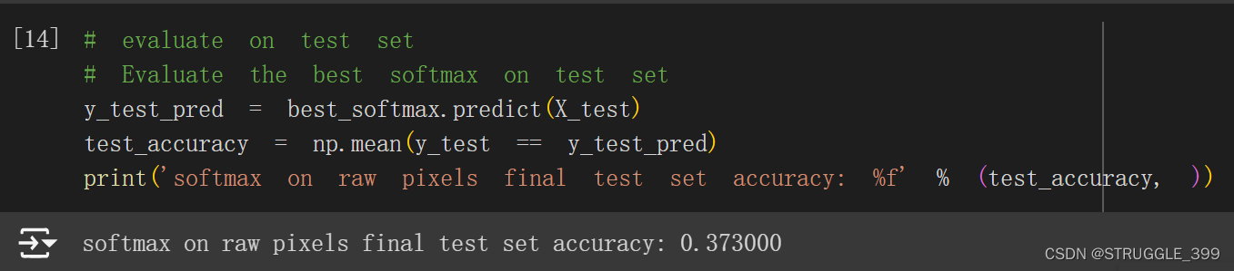
在测试集中测试,获取测试精度为 37.3%。
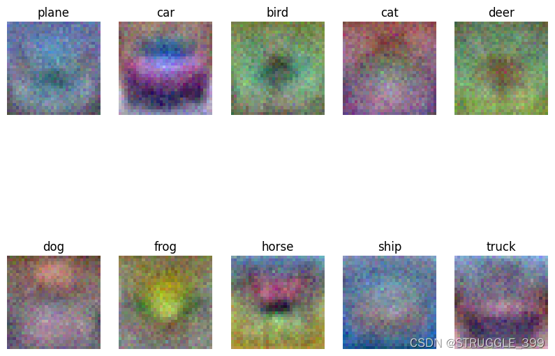
Softmax 分类器学习到的权重可视化如下,结果与 SVM 分类器学习到的权重可视化图相近。
Q4: Two-Layer Neural Network
在本练习中,我们将采用模块化方法实现全连接网络(fully-connected neural network)。我们将为每一层实现一个 forward 和 backward 函数。forward 函数将接收输入、权重和其他参数,并返回输出和 cache 对象,cache 对象中存储了后向传递所需的数据,就像下面这样:
def layer_forward(x, w):
  """ Receive inputs x and weights w """
  # Do some computations ...
  z = # ... some intermediate value
  # Do some more computations ...
  out = # the output

  cache = (x, w, z, out) # Values we need to compute gradients

  return out, cache
后向传递将接收上游导数和 cache 对象,并返回相对于输入和权重的梯度,就像这样:
def layer_backward(dout, cache):
  """
  Receive dout (derivative of loss with respect to outputs) and cache,
  and compute derivative with respect to inputs.
  """
  # Unpack cache values
  x, w, z, out = cache

  # Use values in cache to compute derivatives
  dx = # Derivative of loss with respect to x
  dw = # Derivative of loss with respect to w

  return dx, dw
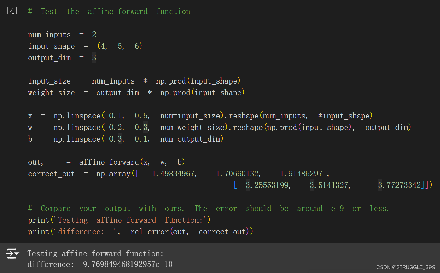
affine layer
affine_forward
首先实现的是仿射层(affine layer)的前向函数,仿射层做的变换为仿射变换,形式为:
y
=
w
x
+
b
y=wx+b
y=wx+b
具体的实现思路为:
- 将 x 变换形状,将每一行延展成一个行向量,最终 x 变换为矩阵,其形状为
(N, D)。 - 通过
np.dot(x, w) + b即可完成仿射变换。
def affine_forward(x, w, b):
    """
    Computes the forward pass for an affine (fully-connected) layer.

    The input x has shape (N, d_1, ..., d_k) and contains a minibatch of N
    examples, where each example x[i] has shape (d_1, ..., d_k). We will
    reshape each input into a vector of dimension D = d_1 * ... * d_k, and
    then transform it to an output vector of dimension M.

    Inputs:
    - x: A numpy array containing input data, of shape (N, d_1, ..., d_k)
    - w: A numpy array of weights, of shape (D, M)
    - b: A numpy array of biases, of shape (M,)

    Returns a tuple of:
    - out: output, of shape (N, M)
    - cache: (x, w, b)
    """
    out = None
    ###########################################################################
    # TODO: Implement the affine forward pass. Store the result in out. You   #
    # will need to reshape the input into rows.                               #
    ###########################################################################
    # *****START OF YOUR CODE (DO NOT DELETE/MODIFY THIS LINE)*****

    out = np.dot(np.reshape(x, (x.shape[0], -1)), w) + b

    # *****END OF YOUR CODE (DO NOT DELETE/MODIFY THIS LINE)*****
    ###########################################################################
    #                             END OF YOUR CODE                            #
    ###########################################################################
    cache = (x, w, b)
    return out, cache
测试结果如下:
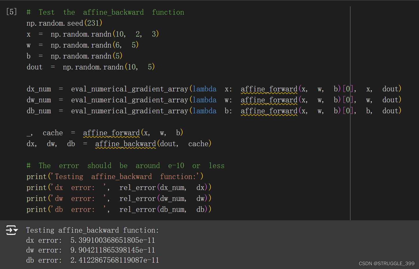
affine_backward
接下来实现的是仿射层(affine layer)的后向函数,仿射层实际的计算公式为:
y
=
x
w
+
b
y=xw+b
y=xw+b
其中 x 为形如 (N, D) 的矩阵, w 为形如 (D, M) 的矩阵,b 为 形如(M, )的行向量,具体计算时会利用广播机制。
下面为梯度推导过程,首先定义几个符号:
X
=
(
x
11
x
12
⋯
x
1
D
x
21
x
22
⋯
x
2
D
⋮
⋮
⋮
x
N
1
x
N
2
⋯
x
N
D
)
W
=
(
w
11
w
12
⋯
w
1
M
w
21
w
22
⋯
w
2
M
⋮
⋮
⋮
w
D
1
w
D
2
⋯
w
D
M
)
Y
=
(
y
11
y
12
⋯
y
1
M
y
21
y
22
⋯
y
2
M
⋮
⋮
⋮
y
N
1
y
N
2
⋯
y
N
M
)
b
=
(
b
1
b
2
⋯
b
M
)
X= \begin{pmatrix} x_{11} &x_{12} &\cdots&x_{1D}\\ x_{21} &x_{22} &\cdots&x_{2D}\\ \vdots &\vdots & &\vdots\\ x_{N1} &x_{N2} & \cdots &x_{ND} \end{pmatrix}\, W= \begin{pmatrix} w_{11} &w_{12} &\cdots&w_{1M}\\ w_{21} &w_{22} &\cdots&w_{2M}\\ \vdots &\vdots & &\vdots\\ w_{D1} &w_{D2} & \cdots &w_{DM} \end{pmatrix}\, Y= \begin{pmatrix} y_{11} &y_{12} &\cdots&y_{1M}\\ y_{21} &y_{22} &\cdots&y_{2M}\\ \vdots &\vdots & &\vdots\\ y_{N1} &y_{N2} & \cdots &y_{NM} \end{pmatrix} \\\\ b= \begin{pmatrix} b_1&b_2&\cdots&b_M \end{pmatrix}
X=
x11x21⋮xN1x12x22⋮xN2⋯⋯⋯x1Dx2D⋮xND
W=
w11w21⋮wD1w12w22⋮wD2⋯⋯⋯w1Mw2M⋮wDM
Y=
y11y21⋮yN1y12y22⋮yN2⋯⋯⋯y1My2M⋮yNM
b=(b1b2⋯bM)
根据仿射变换的公式,我们不难得到:
y
i
j
=
∑
k
x
i
k
w
k
j
+
b
j
y_{ij}=\sum_k x_{ik}w_{kj} + b_j
yij=k∑xikwkj+bj
其中
1
≤
i
≤
N
,
1
≤
j
≤
M
1\le i\le N,1\le j\le M
1≤i≤N,1≤j≤M,我们可以得到,
y
i
j
y_{ij}
yij 与 矩阵
X
X
X 的第 i 行、矩阵
W
W
W 的第 j 列以及向量
b
b
b 的第 j 个分量有关,因此:
∂
y
i
j
∂
x
i
k
=
w
k
j
,
∂
y
i
j
∂
x
k
j
=
x
i
k
,
∂
y
i
j
∂
b
j
=
1
\frac{\partial y_{ij}}{\partial x_{ik}}=w_{kj}, \frac{\partial y_{ij}}{\partial x_{kj}}=x_{ik}, \frac{\partial y_{ij}}{\partial b_{j}}=1
∂xik∂yij=wkj,∂xkj∂yij=xik,∂bj∂yij=1
根据链式法则,我们可以得到 dx、dw、db 的梯度:
∂
L
∂
b
j
=
∑
k
d
y
k
j
(
1
≤
k
≤
M
)
\frac{\partial L}{\partial b_j}=\sum_kdy_{kj}\,(1\le k\le M)
∂bj∂L=k∑dykj(1≤k≤M)
∂ L ∂ x i j = ∑ k w j k d y i k ( 1 ≤ k ≤ M ) \frac{\partial L}{\partial x_{ij}}=\sum_k w_{jk}dy_{ik}\,(1\le k\le M) ∂xij∂L=k∑wjkdyik(1≤k≤M)
∂ L ∂ w i j = ∑ k x k i d y k j ( 1 ≤ k ≤ N ) \frac{\partial L}{\partial w_{ij}}=\sum_k x_{ki}dy_{kj}\,(1\le k\le N) ∂wij∂L=k∑xkidykj(1≤k≤N)
根据以上分析,我们可以得到 dx、dw、db 的计算方法如下:
∂
L
∂
X
=
d
Y
∗
W
T
,
∂
L
∂
W
=
X
T
∗
d
Y
\frac{\partial L}{\partial X}=dY * W^T,\frac{\partial L}{\partial W}=X^T * dY
∂X∂L=dY∗WT,∂W∂L=XT∗dY
∂ L ∂ b = ( ∑ k d y k 1 ∑ k d y k 2 ⋯ ∑ k d y k M ) \frac{\partial L}{\partial b}= \begin{pmatrix} \sum_kdy_{k1} & \sum_kdy_{k2} &\cdots &\sum_kdy_{kM} \end{pmatrix} ∂b∂L=(∑kdyk1∑kdyk2⋯∑kdykM)
有了计算公式后,具体实现如下:
def affine_backward(dout, cache):
    """
    Computes the backward pass for an affine layer.

    Inputs:
    - dout: Upstream derivative, of shape (N, M)
    - cache: Tuple of:
      - x: Input data, of shape (N, d_1, ... d_k)
      - w: Weights, of shape (D, M)
      - b: Biases, of shape (M,)

    Returns a tuple of:
    - dx: Gradient with respect to x, of shape (N, d1, ..., d_k)
    - dw: Gradient with respect to w, of shape (D, M)
    - db: Gradient with respect to b, of shape (M,)
    """
    x, w, b = cache
    dx, dw, db = None, None, None
    ###########################################################################
    # TODO: Implement the affine backward pass.                               #
    ###########################################################################
    # *****START OF YOUR CODE (DO NOT DELETE/MODIFY THIS LINE)*****

    dx = np.reshape(np.dot(dout, w.T), x.shape)
    dw = np.dot(np.reshape(x, (x.shape[0], -1)).T, dout)
    db = np.sum(dout, axis=0)

    # *****END OF YOUR CODE (DO NOT DELETE/MODIFY THIS LINE)*****
    ###########################################################################
    #                             END OF YOUR CODE                            #
    ###########################################################################
    return dx, dw, db
梯度测试如下:
ReLU activation layer
ReLU 激活函数的公式如下:
σ
(
x
)
=
max
(
0
,
x
)
\sigma(x)=\max(0, x)
σ(x)=max(0,x)
ReLU 函数的梯度为:
d
σ
d
x
=
{
0
if
x
≤
0
1
if
x
>
0
\frac{d\sigma}{dx}= \begin{cases} 0\, &\text{if } x\le 0\\ 1\, &\text{if } x > 0 \end{cases}
dxdσ={01if x≤0if x>0
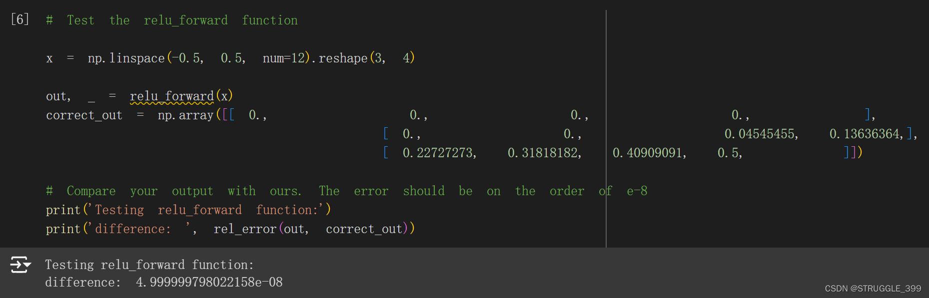
relu_forward
ReLU 层的前向函数实现特别简单,就是通过 np.maximum(0, x) 即可实现 ReLU 激活函数。
def relu_forward(x):
    """
    Computes the forward pass for a layer of rectified linear units (ReLUs).

    Input:
    - x: Inputs, of any shape

    Returns a tuple of:
    - out: Output, of the same shape as x
    - cache: x
    """
    out = None
    ###########################################################################
    # TODO: Implement the ReLU forward pass.                                  #
    ###########################################################################
    # *****START OF YOUR CODE (DO NOT DELETE/MODIFY THIS LINE)*****

    out = np.maximum(0, x)

    # *****END OF YOUR CODE (DO NOT DELETE/MODIFY THIS LINE)*****
    ###########################################################################
    #                             END OF YOUR CODE                            #
    ###########################################################################
    cache = x
    return out, cache
ReLU 前向函数测试如下:
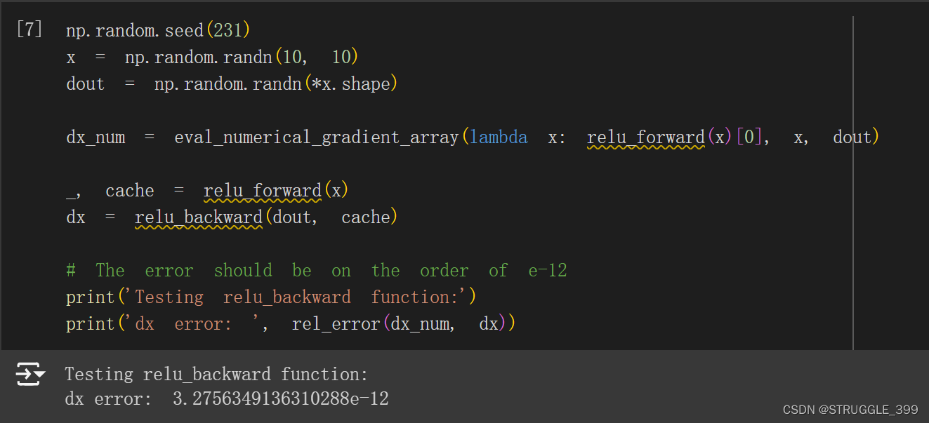
relu_backward
根据 ReLU 激活函数的导数公式,可得 ReLU 层的反向函数实现思路为:
- 通过
x > 0生成一个布尔矩阵。 dout * (x > 0)就是 dx,这一步操作是一个过滤功能,将原来x < 0的元素对应的梯度置零。
def relu_backward(dout, cache):
    """
    Computes the backward pass for a layer of rectified linear units (ReLUs).

    Input:
    - dout: Upstream derivatives, of any shape
    - cache: Input x, of same shape as dout

    Returns:
    - dx: Gradient with respect to x
    """
    dx, x = None, cache
    ###########################################################################
    # TODO: Implement the ReLU backward pass.                                 #
    ###########################################################################
    # *****START OF YOUR CODE (DO NOT DELETE/MODIFY THIS LINE)*****

    dx = dout * (x > 0)

    # *****END OF YOUR CODE (DO NOT DELETE/MODIFY THIS LINE)*****
    ###########################################################################
    #                             END OF YOUR CODE                            #
    ###########################################################################
    return dx
ReLU 层后向函数测试如下:
Inline Question 1
我们只要求你实现 ReLU,但在神经网络中可以使用多种不同的激活函数,每种函数都有其优缺点。特别是,激活函数常见的一个问题是在反向传播过程中梯度流为零(或接近零)。以下哪些激活函数存在这个问题?如果在一维情况下考虑这些函数,哪些类型的输入会导致这种行为?
- Sigmoid
- ReLU
- Leaky ReLU
【答】1、2。
-
Sigmoid 激活函数形式为:
σ ( x ) = 1 1 + e − x \sigma(x)=\frac{1}{1+e^{-x}} σ(x)=1+e−x1
Sigmoid 函数图像如下所示,当 x 的绝对值充分大时,其梯度接近于零。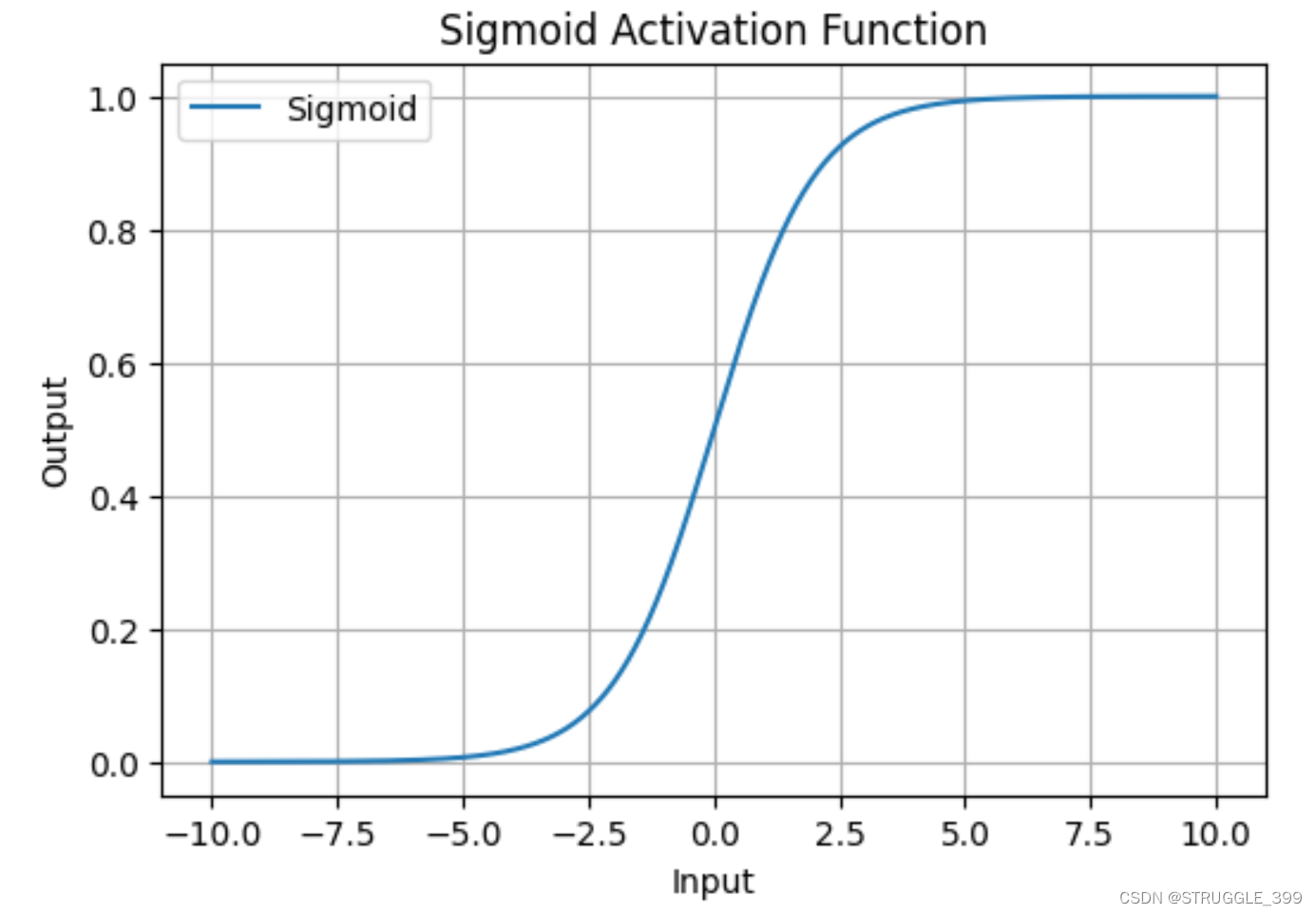
-
ReLU 激活函数形式为:
σ ( x ) = max ( 0 , x ) \sigma(x)=\max(0, x) σ(x)=max(0,x)
在 x 的正半轴中,ReLU 函数不会饱和,因此梯度不会为零,而在 x 的负半轴中,ReLU 函数的梯度为零。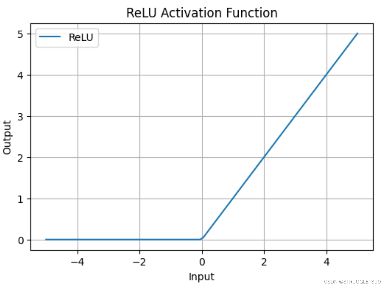
-
Leaky ReLU 激活函数形式为:
σ ( x ) = max ( α x , x ) \sigma(x)=\max(\alpha x,x) σ(x)=max(αx,x)
Leaky ReLU 函数不会饱和,因此梯度不会为零(或接近零)。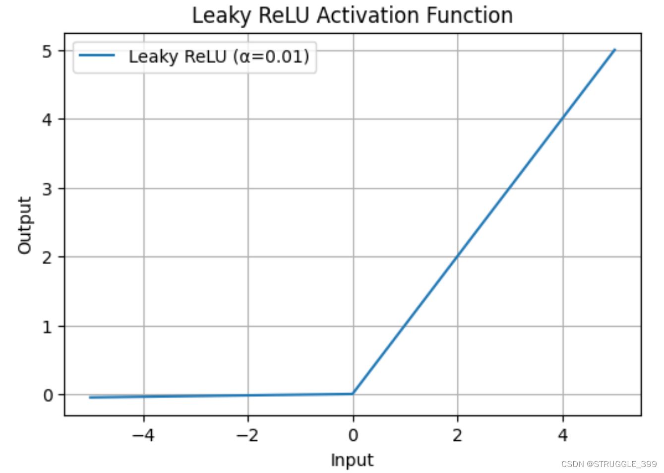
“Sandwich” layers
所谓的 “三明治” 层,就是将若干层组合起来形成一个更大的层,例如仿射层(affine layer)后跟一个 ReLU 非线性层。实现思路如下:
affine_relu_forward可以用affine_forward和relu_forward实现。affine_relu_backward可以用affine_backward和relu_backward实现。
affine_relu_forward
注意调用次序,首先调用 affine_forward,在调用 relu_forward。
def affine_relu_forward(x, w, b):
    """
    Convenience layer that perorms an affine transform followed by a ReLU

    Inputs:
    - x: Input to the affine layer
    - w, b: Weights for the affine layer

    Returns a tuple of:
    - out: Output from the ReLU
    - cache: Object to give to the backward pass
    """
    a, fc_cache = affine_forward(x, w, b)
    out, relu_cache = relu_forward(a)
    cache = (fc_cache, relu_cache)
    return out, cache
affine_relu_backward
注意调用顺序,首先调用 relu_backward,再调用 affine_backward 。
def affine_relu_backward(dout, cache):
    """
    Backward pass for the affine-relu convenience layer
    """
    fc_cache, relu_cache = cache
    da = relu_backward(dout, relu_cache)
    dx, dw, db = affine_backward(da, fc_cache)
    return dx, dw, db
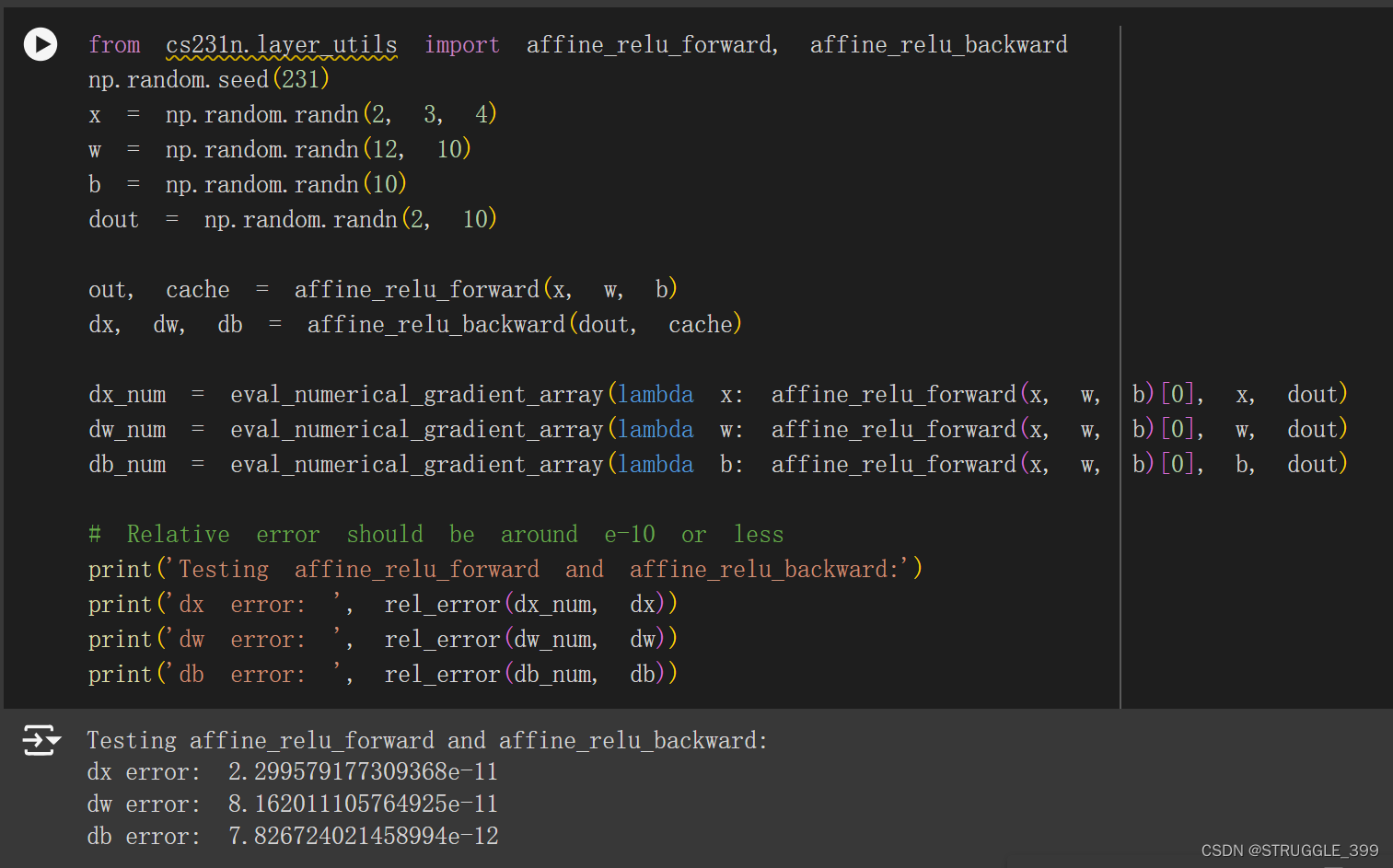
测试结果如下:
loss layers
loss 层的 softmax 层、svm 层的损失、梯度的计算与前面的 softmax_loss、svm_loss 的实现非常类似,区别在于:
- softmax 层、svm 层的输入 x 就是得分矩阵
scores(不再是 x 和 参数 w、b)。 - 得益于反向传播算法,梯度的计算不再需要直接计算相对于神经网络的输入梯度,只需要相对于得分矩阵的梯度。
softmax layer
loss 的计算同 Q3 的 softmax_loss_vectorized 计算方式相同,而梯度的计算则更为简单,只需要计算损失相对于得分的梯度。Softmax 分类器的代价函数为:
L
=
1
N
∑
i
[
log
(
∑
j
e
f
(
x
i
,
W
)
j
)
−
f
(
x
i
,
W
)
y
i
]
L=\frac{1}{N}\sum_i [\log(\sum_j e^{f(x_i,W)_j})-f(x_i,W)_{y_i}]
L=N1i∑[log(j∑ef(xi,W)j)−f(xi,W)yi]
其中,x[i, j] 就是
f
(
x
i
,
W
)
j
f(x_i,W)_j
f(xi,W)j。因此梯度推导如下:
KaTeX parse error: Undefined control sequence: \part at position 8: \frac{\̲p̲a̲r̲t̲ ̲L}{\part x_{ij}…
整理后可得:
∂
L
∂
x
i
j
=
{
1
N
p
i
j
if
j
≠
y
i
1
N
(
p
i
j
−
1
)
if
j
=
y
i
\frac{\partial L}{\partial x_{ij}}= \begin{cases} \frac{1}{N}p_{ij}&\text{ if } j\ne y_i\\ \frac{1}{N}(p_{ij}-1)&\text{ if } j=y_i \end{cases}
∂xij∂L={N1pijN1(pij−1) if j=yi if j=yi
因此在计算完损失后,通过 p[range(num_train), y] -= 1 统一形式,之后 p / N 即为所求的损失对得分的梯度值。
def softmax_loss(x, y):
    """
    Computes the loss and gradient for softmax classification.

    Inputs:
    - x: Input data, of shape (N, C) where x[i, j] is the score for the jth
      class for the ith input.
    - y: Vector of labels, of shape (N,) where y[i] is the label for x[i] and
      0 <= y[i] < C

    Returns a tuple of:
    - loss: Scalar giving the loss
    - dx: Gradient of the loss with respect to x
    """
    loss, dx = None, None

    ###########################################################################
    # TODO: Copy over your solution from A1.
    ###########################################################################
    # *****START OF YOUR CODE (DO NOT DELETE/MODIFY THIS LINE)*****

    N, C = x.shape
    x = x - np.max(x, axis=1, keepdims=True) # 保证数值稳定性
    p = np.exp(x) / np.sum(np.exp(x), axis=1, keepdims=True)
    loss = np.sum(-np.log(p[range(N), y])) / N

    p[range(N), y] -= 1
    dx = p / num_train

    # *****END OF YOUR CODE (DO NOT DELETE/MODIFY THIS LINE)*****
    ###########################################################################
    #                             END OF YOUR CODE                            #
    ###########################################################################
    return loss, dx
svm layer
loss 的计算同 Q2 的 svm_loss_vectorized 计算方式相同,同 softmax layer 一样,只需要计算损失相对于得分的梯度。svm 的代价函数定义为:
L
=
1
N
∑
i
∑
j
≠
y
i
max
(
0
,
s
j
−
s
y
i
+
Δ
)
=
1
N
∑
i
∑
j
≠
y
i
max
(
0
,
f
(
x
i
,
W
)
j
−
f
(
x
i
,
W
)
y
i
+
Δ
)
\begin{aligned} L&=\frac{1}{N}\sum_i\sum_{j\ne y_i}\max(0,s_j-s_{y_i}+\Delta)\\ &=\frac{1}{N}\sum_i\sum_{j\ne y_i}\max(0,f(x_i,W)_j-f(x_i,W)_{y_i}+\Delta) \end{aligned}
L=N1i∑j=yi∑max(0,sj−syi+Δ)=N1i∑j=yi∑max(0,f(xi,W)j−f(xi,W)yi+Δ)
其中,x[i, j] 就是
f
(
x
i
,
W
)
j
f(x_i,W)_j
f(xi,W)j。
当
j
≠
y
i
j\ne y_i
j=yi 时,
∂
L
∂
x
i
j
=
{
1
N
if
f
(
x
i
,
W
)
j
−
f
(
x
i
,
W
)
y
i
+
Δ
>
0
0
otherwise
\frac{\partial L}{\partial x_{ij}}= \begin{cases} \frac{1}{N}&\text{if }f(x_i,W)_j-f(x_i,W)_{y_i}+\Delta>0\\ 0&\text{otherwise} \end{cases}
∂xij∂L={N10if f(xi,W)j−f(xi,W)yi+Δ>0otherwise
当
j
=
y
i
j=y_i
j=yi 时,
∂
L
∂
x
i
y
i
=
∑
j
≠
y
i
∂
L
∂
x
i
j
\frac{\partial L}{\partial x_{iy_i}}=\sum_{j\ne y_i}\frac{\partial L}{\partial x_{ij}}
∂xiyi∂L=j=yi∑∂xij∂L
因此梯度计算的实现思路为:
margins[margins > 0] = 1,将margins中所有大于零元素置为 1。margins[range(N), y] = -np.sum(margins, axis=1)。dx = margins / N。
def svm_loss(x, y):
    """
    Computes the loss and gradient using for multiclass SVM classification.

    Inputs:
    - x: Input data, of shape (N, C) where x[i, j] is the score for the jth
      class for the ith input.
    - y: Vector of labels, of shape (N,) where y[i] is the label for x[i] and
      0 <= y[i] < C

    Returns a tuple of:
    - loss: Scalar giving the loss
    - dx: Gradient of the loss with respect to x
    """
    loss, dx = None, None

    ###########################################################################
    # TODO: Copy over your solution from A1.
    ###########################################################################
    # *****START OF YOUR CODE (DO NOT DELETE/MODIFY THIS LINE)*****

    N, C = x.shape
    # 正确分类的得分
    correct_class_scores = x[range(N), y].reshape(N, 1)
    margins = np.maximum(0, x - correct_class_scores + 1)
    margins[range(N), y] = 0
    loss = np.sum(margins) / N

    margins[margins > 0] = 1
    margins[range(N), y] = -np.sum(margins, axis=1)
    dx = margins / N

    # *****END OF YOUR CODE (DO NOT DELETE/MODIFY THIS LINE)*****
    ###########################################################################
    #                             END OF YOUR CODE                            #
    ###########################################################################
    return loss, dx
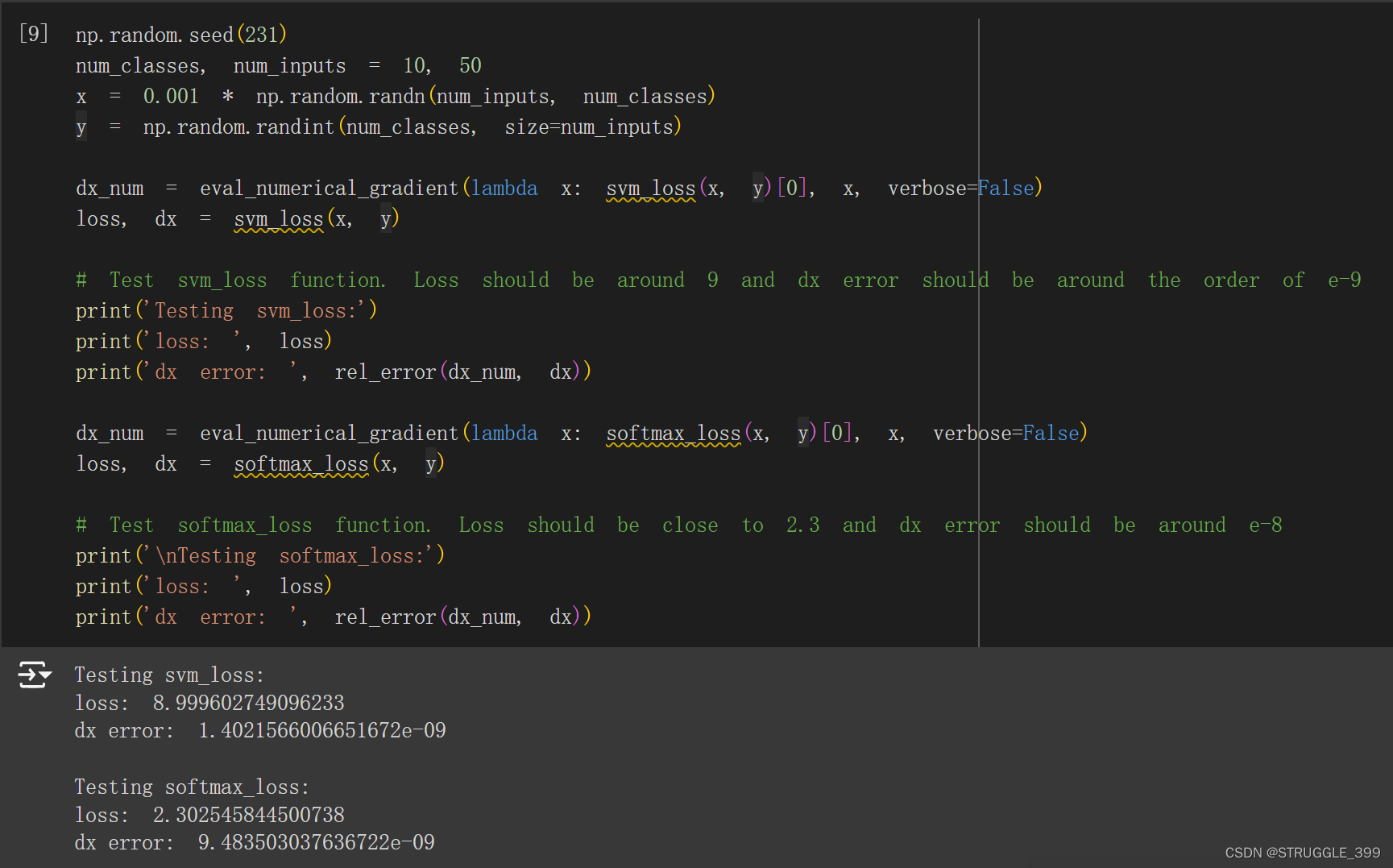
测试结果如下:
TwoLayerNet
init
__init__() 方法为 TwoLayerNet 的构造函数,主要用于初始化模型的参数。
def __init__(
    self,
    input_dim=3 * 32 * 32,
    hidden_dim=100,
    num_classes=10,
    weight_scale=1e-3,
    reg=0.0,
):
    """
    Initialize a new network.

    Inputs:
    - input_dim: An integer giving the size of the input
    - hidden_dim: An integer giving the size of the hidden layer
    - num_classes: An integer giving the number of classes to classify
    - weight_scale: Scalar giving the standard deviation for random
      initialization of the weights.
    - reg: Scalar giving L2 regularization strength.
    """
    self.params = {}
    self.reg = reg

    ############################################################################
    # TODO: Initialize the weights and biases of the two-layer net. Weights    #
    # should be initialized from a Gaussian centered at 0.0 with               #
    # standard deviation equal to weight_scale, and biases should be           #
    # initialized to zero. All weights and biases should be stored in the      #
    # dictionary self.params, with first layer weights                         #
    # and biases using the keys 'W1' and 'b1' and second layer                 #
    # weights and biases using the keys 'W2' and 'b2'.                         #
    ############################################################################
    # *****START OF YOUR CODE (DO NOT DELETE/MODIFY THIS LINE)*****

    self.params['W1'] = np.random.randn(input_dim, hidden_dim) * weight_scale
    self.params['b1'] = np.zeros(hidden_dim)
    self.params['W2'] = np.random.randn(hidden_dim, num_classes) * weight_scale
    self.params['b2'] = np.zeros(num_classes)

    # *****END OF YOUR CODE (DO NOT DELETE/MODIFY THIS LINE)*****
    ############################################################################
    #                             END OF YOUR CODE                             #
    ############################################################################
loss
loss 函数用于计算模型的损失以及损失相对于每个参数的梯度,梯度存放于 grads 字典中,键名与参数名对应。loss 函数就是执行模型的前向传播和反向传播两个部分,前向传播计算损失,反向传播计算损失相对于各参数的梯度,具体实现如下:
def loss(self, X, y=None):
    """
    Compute loss and gradient for a minibatch of data.

    Inputs:
    - X: Array of input data of shape (N, d_1, ..., d_k)
    - y: Array of labels, of shape (N,). y[i] gives the label for X[i].

    Returns:
    If y is None, then run a test-time forward pass of the model and return:
    - scores: Array of shape (N, C) giving classification scores, where
      scores[i, c] is the classification score for X[i] and class c.

    If y is not None, then run a training-time forward and backward pass and
    return a tuple of:
    - loss: Scalar value giving the loss
    - grads: Dictionary with the same keys as self.params, mapping parameter
      names to gradients of the loss with respect to those parameters.
    """
    scores = None
    ############################################################################
    # TODO: Implement the forward pass for the two-layer net, computing the    #
    # class scores for X and storing them in the scores variable.              #
    ############################################################################
    # *****START OF YOUR CODE (DO NOT DELETE/MODIFY THIS LINE)*****

    a, cache1 = affine_relu_forward(X, self.params['W1'], self.params['b1'])
    scores, cache2 = affine_forward(a, self.params['W2'], self.params['b2'])

    # *****END OF YOUR CODE (DO NOT DELETE/MODIFY THIS LINE)*****
    ############################################################################
    #                             END OF YOUR CODE                             #
    ############################################################################

    # If y is None then we are in test mode so just return scores
    if y is None:
        return scores

    loss, grads = 0, {}
    ############################################################################
    # TODO: Implement the backward pass for the two-layer net. Store the loss  #
    # in the loss variable and gradients in the grads dictionary. Compute data #
    # loss using softmax, and make sure that grads[k] holds the gradients for  #
    # self.params[k]. Don't forget to add L2 regularization!                   #
    #                                                                          #
    # NOTE: To ensure that your implementation matches ours and you pass the   #
    # automated tests, make sure that your L2 regularization includes a factor #
    # of 0.5 to simplify the expression for the gradient.                      #
    ############################################################################
    # *****START OF YOUR CODE (DO NOT DELETE/MODIFY THIS LINE)*****

    loss, dscores = softmax_loss(scores, y)
    # 加上 L2 正则化损失
    loss += 0.5 * self.reg * (np.sum(np.square(self.params['W1'])) + np.sum(np.square(self.params['W2'])))

    dx, grads['W2'], grads['b2'] = affine_backward(dscores, cache2)
    grads['W1'], grads['b1'] = affine_relu_backward(dx, cache1)[1:]

    # 梯度加上正则化项的梯度
    grads['W1'] += self.reg * self.params['W1']
    grads['W2'] += self.reg * self.params['W2']

    # *****END OF YOUR CODE (DO NOT DELETE/MODIFY THIS LINE)*****
    ############################################################################
    #                             END OF YOUR CODE                             #
    ############################################################################

    return loss, grads
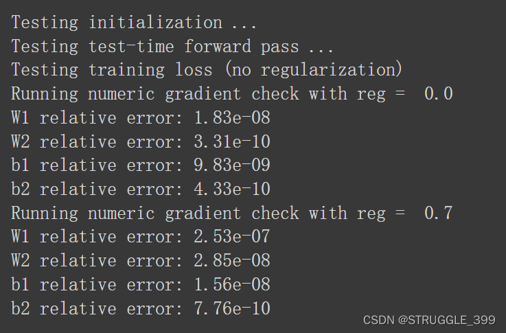
运行测试,测试结果如下:
Solver
作业一中提供了一个 Solver 工具类,用于模型的训练,Solver 类的构造函数中可以传递许多参数,其中必要的参数为 model 对象、训练数据 data,还有许多可选的参数,详情请见作业一的 cs231n/solver.py 文件。
input_size = 32 * 32 * 3
hidden_size = 50
num_classes = 10
model = TwoLayerNet(input_size, hidden_size, num_classes)
solver = None

##############################################################################
# TODO: Use a Solver instance to train a TwoLayerNet that achieves about 36% #
# accuracy on the validation set.                                            #
##############################################################################
# *****START OF YOUR CODE (DO NOT DELETE/MODIFY THIS LINE)*****

solver = Solver(model, data, optim_config = {'learning_rate': 1e-3})
solver.train()

# *****END OF YOUR CODE (DO NOT DELETE/MODIFY THIS LINE)*****
##############################################################################
#                             END OF YOUR CODE                               #
##############################################################################
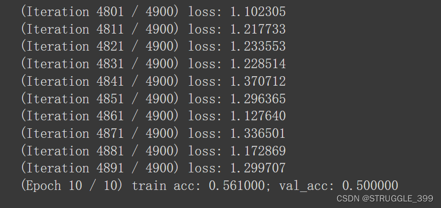
测试结果如下,最终的验证精度达到了 50%:
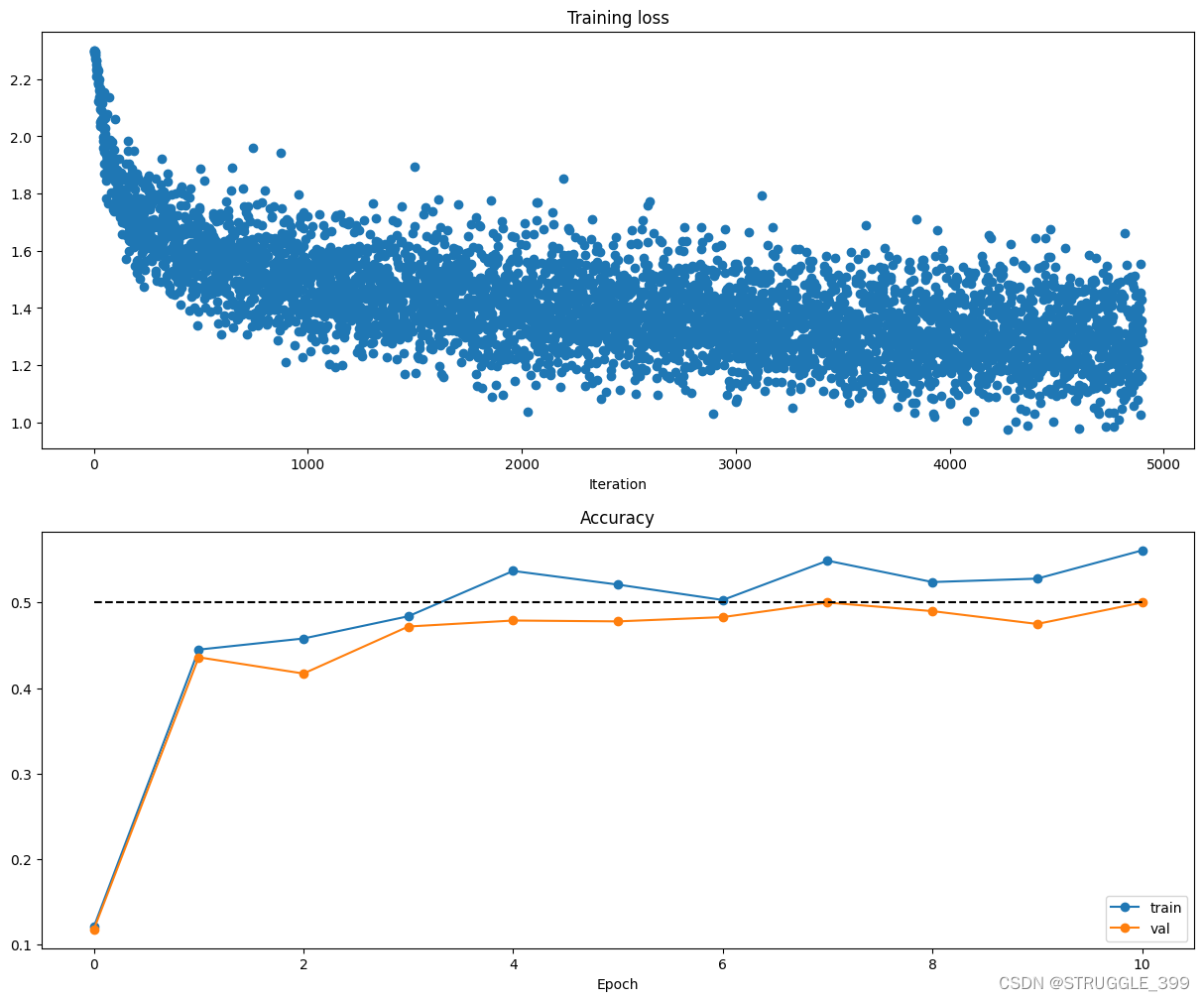
损失、训练精度/验证精度随着迭代次数(或epoch)的变化图如下。
接下来将 TwoLayerNet 学习到的第一层权重进行可视化:
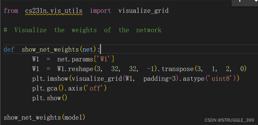
权重可视化的结果如下:

两层神经网络学习到的模板比线性分类器 softmax/svm 学习的模板更多,这里学习的模板数量为50个,因为隐藏层的大小/维度为50,上面的可视化结果就是这50个模板。
最后的任务就是进行超参数调整(Hyperparameter tuning)了,我们在前面的学习率设定为固定学习率0.001时,模型已经获得50%的验证精度,在超参数调整过程中,发现当正则化参数大于10时,模型的训练精度、验证精度都下降的非常明显,说明模型发生欠拟合(Underfitting)。具体的超参数调整代码如下,
best_model = None

#################################################################################
# TODO: Tune hyperparameters using the validation set. Store your best trained  #
# model in best_model.                                                          #
#                                                                               #
# To help debug your network, it may help to use visualizations similar to the  #
# ones we used above; these visualizations will have significant qualitative    #
# differences from the ones we saw above for the poorly tuned network.          #
#                                                                               #
# Tweaking hyperparameters by hand can be fun, but you might find it useful to  #
# write code to sweep through possible combinations of hyperparameters          #
# automatically like we did on thexs previous exercises.                          #
#################################################################################
# *****START OF YOUR CODE (DO NOT DELETE/MODIFY THIS LINE)*****
best_val = -1
best_params = None

# learning_rates = [1e-4, 3e-4, 1e-3, 3e-3]
learning_rates = [1e-3, 2e-3]
regularization_strengths = [1e-3, 1e-2, 1e-1, 1, 1e1]

for lr in learning_rates:
  for reg in regularization_strengths:
    print('learing rate=%f, regularization strength=%f' % (lr, reg))
    model = TwoLayerNet(input_size, hidden_size, num_classes, reg=reg)
    solver = Solver(model, data, optim_config={'learning_rate': lr})
    solver.train()
    if solver.best_val_acc > best_val:
      best_val = solver.best_val_acc
      best_params = (lr, reg)
      best_model = model

    # visualize training loss and train / val accuracy
    plt.subplot(2, 1, 1)
    plt.title('Training loss(learing rate=%f, regularization strength=%f)' % (lr, reg))
    plt.plot(solver.loss_history, 'o')
    plt.xlabel('Iteration')

    plt.subplot(2, 1, 2)
    plt.title('Accuracy(learing rate=%f, regularization strength=%f)' % (lr, reg))
    plt.plot(solver.train_acc_history, '-o', label='train')
    plt.plot(solver.val_acc_history, '-o', label='val')
    plt.plot([0.5] * len(solver.val_acc_history), 'k--')
    plt.xlabel('Epoch')
    plt.legend(loc='lower right')
    plt.gcf().set_size_inches(15, 12)
    plt.show()


print('best validation accuracy achieved during cross-validation: %f' % best_val)
print('best learning rate=%f, best regularization strengths=%f' % best_params)

# *****END OF YOUR CODE (DO NOT DELETE/MODIFY THIS LINE)*****
################################################################################
#                              END OF YOUR CODE                                #
################################################################################
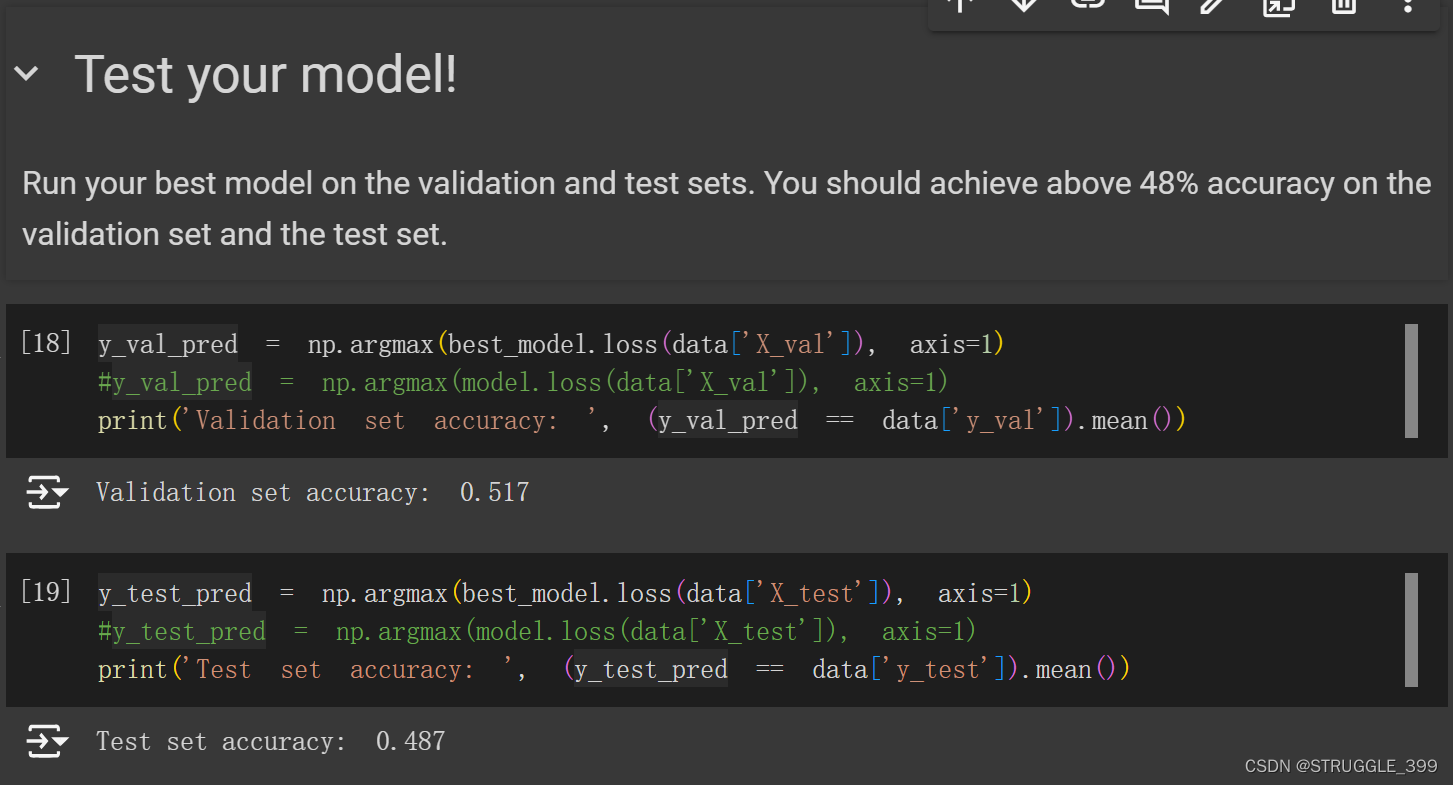
测试的结果如下,最终得到的最好的超参数组合为:(learning_rate, regularization_strength) = (0.001, 0.01)。最好的验证集精度为 51.7%。
best validation accuracy achieved during cross-validation: 0.517000
best learning rate=0.001000, best regularization strengths=0.010000
最终模型在测试集中的准确率为 48.7%。
Inline Question 2
现在您已经训练了一个神经网络分类器,但您可能会发现测试准确率远远低于训练准确率。我们可以通过哪些方法来缩小这一差距?请选所有适用的方法。
- 在更大的数据集上进行训练。
- 添加更多隐藏单元。
- 增加正则化强度。
- 以上都不是。
【答】1、3。
测试准确率远远低于训练准确率表明神经网络发生了过拟合(Overfitting)。
- 在更大的数据集上训练,一定程度上可以缓解过拟合现象。
- 添加更多隐藏单元则会使得模型更深,更加复杂,更容易产生过拟合现象。
- 增加正则化强度可以一定程度上使模型更简单,避免过拟合现象。
Q5: Higher Level Representations: Image Features
我们已经看到,通过在输入图像的像素上训练线性分类器,我们可以在图像分类任务中取得合理的性能。在本练习中,我们将展示如何不根据原始像素,而是根据原始像素计算出的特征来训练线性分类器,从而提高分类性能。
# Use the validation set to tune the learning rate and regularization strength

from cs231n.classifiers.linear_classifier import LinearSVM

learning_rates = [1e-4, 3e-4, 1e-3, 3e-3, 1e-2, 3e-2]
regularization_strengths = [1e-6, 1e-5, 1e-4, 1e-3, 1e-2, 1e-1, 0, 1]

results = {}
best_val = -1
best_svm = None

################################################################################
# TODO:                                                                        #
# Use the validation set to set the learning rate and regularization strength. #
# This should be identical to the validation that you did for the SVM; save    #
# the best trained classifer in best_svm. You might also want to play          #
# with different numbers of bins in the color histogram. If you are careful    #
# you should be able to get accuracy of near 0.44 on the validation set.       #
################################################################################
# *****START OF YOUR CODE (DO NOT DELETE/MODIFY THIS LINE)*****

for lr in learning_rates:
  for reg in regularization_strengths:
    svm = LinearSVM()
    loss_hist = svm.train(X_train_feats, y_train, learning_rate=lr, reg=reg,
                      num_iters=1500, verbose=True)
    y_train_pred = svm.predict(X_train_feats)
    y_val_pred = svm.predict(X_val_feats)
    training_accuracy = np.mean(y_train == y_train_pred)
    validation_accuracy = np.mean(y_val == y_val_pred)
    results[(lr, reg)] = (training_accuracy, validation_accuracy)

    if best_val < validation_accuracy:
      best_val = validation_accuracy
      best_svm = svm
# *****END OF YOUR CODE (DO NOT DELETE/MODIFY THIS LINE)*****

# Print out results.
for lr, reg in sorted(results):
    train_accuracy, val_accuracy = results[(lr, reg)]
    print('lr %e reg %e train accuracy: %f val accuracy: %f' % (
                lr, reg, train_accuracy, val_accuracy))

print('best validation accuracy achieved: %f' % best_val)
测试结果如下:
lr 1.000000e-04 reg 0.000000e+00 train accuracy: 0.450694 val accuracy: 0.444000
lr 1.000000e-04 reg 1.000000e-06 train accuracy: 0.449633 val accuracy: 0.445000
lr 1.000000e-04 reg 1.000000e-05 train accuracy: 0.450959 val accuracy: 0.441000
lr 1.000000e-04 reg 1.000000e-04 train accuracy: 0.450837 val accuracy: 0.446000
lr 1.000000e-04 reg 1.000000e-03 train accuracy: 0.450714 val accuracy: 0.443000
lr 1.000000e-04 reg 1.000000e-02 train accuracy: 0.451980 val accuracy: 0.448000
lr 1.000000e-04 reg 1.000000e-01 train accuracy: 0.451429 val accuracy: 0.443000
lr 1.000000e-04 reg 1.000000e+00 train accuracy: 0.449531 val accuracy: 0.445000
lr 3.000000e-04 reg 0.000000e+00 train accuracy: 0.480020 val accuracy: 0.474000
lr 3.000000e-04 reg 1.000000e-06 train accuracy: 0.480102 val accuracy: 0.472000
lr 3.000000e-04 reg 1.000000e-05 train accuracy: 0.480245 val accuracy: 0.469000
lr 3.000000e-04 reg 1.000000e-04 train accuracy: 0.480102 val accuracy: 0.470000
lr 3.000000e-04 reg 1.000000e-03 train accuracy: 0.479490 val accuracy: 0.473000
lr 3.000000e-04 reg 1.000000e-02 train accuracy: 0.480490 val accuracy: 0.471000
lr 3.000000e-04 reg 1.000000e-01 train accuracy: 0.479531 val accuracy: 0.471000
lr 3.000000e-04 reg 1.000000e+00 train accuracy: 0.476939 val accuracy: 0.469000
lr 1.000000e-03 reg 0.000000e+00 train accuracy: 0.501408 val accuracy: 0.490000
lr 1.000000e-03 reg 1.000000e-06 train accuracy: 0.501204 val accuracy: 0.482000
lr 1.000000e-03 reg 1.000000e-05 train accuracy: 0.501776 val accuracy: 0.484000
lr 1.000000e-03 reg 1.000000e-04 train accuracy: 0.500939 val accuracy: 0.488000
lr 1.000000e-03 reg 1.000000e-03 train accuracy: 0.501633 val accuracy: 0.485000
lr 1.000000e-03 reg 1.000000e-02 train accuracy: 0.500510 val accuracy: 0.486000
lr 1.000000e-03 reg 1.000000e-01 train accuracy: 0.500367 val accuracy: 0.484000
lr 1.000000e-03 reg 1.000000e+00 train accuracy: 0.490245 val accuracy: 0.479000
lr 3.000000e-03 reg 0.000000e+00 train accuracy: 0.509510 val accuracy: 0.491000
lr 3.000000e-03 reg 1.000000e-06 train accuracy: 0.508755 val accuracy: 0.492000
lr 3.000000e-03 reg 1.000000e-05 train accuracy: 0.509816 val accuracy: 0.495000
lr 3.000000e-03 reg 1.000000e-04 train accuracy: 0.510449 val accuracy: 0.506000
lr 3.000000e-03 reg 1.000000e-03 train accuracy: 0.510816 val accuracy: 0.493000
lr 3.000000e-03 reg 1.000000e-02 train accuracy: 0.509673 val accuracy: 0.490000
lr 3.000000e-03 reg 1.000000e-01 train accuracy: 0.508286 val accuracy: 0.493000
lr 3.000000e-03 reg 1.000000e+00 train accuracy: 0.491898 val accuracy: 0.469000
lr 1.000000e-02 reg 0.000000e+00 train accuracy: 0.508510 val accuracy: 0.495000
lr 1.000000e-02 reg 1.000000e-06 train accuracy: 0.511102 val accuracy: 0.493000
lr 1.000000e-02 reg 1.000000e-05 train accuracy: 0.509061 val accuracy: 0.501000
lr 1.000000e-02 reg 1.000000e-04 train accuracy: 0.511857 val accuracy: 0.494000
lr 1.000000e-02 reg 1.000000e-03 train accuracy: 0.511347 val accuracy: 0.501000
lr 1.000000e-02 reg 1.000000e-02 train accuracy: 0.510429 val accuracy: 0.490000
lr 1.000000e-02 reg 1.000000e-01 train accuracy: 0.507592 val accuracy: 0.506000
lr 1.000000e-02 reg 1.000000e+00 train accuracy: 0.488551 val accuracy: 0.476000
lr 3.000000e-02 reg 0.000000e+00 train accuracy: 0.502694 val accuracy: 0.469000
lr 3.000000e-02 reg 1.000000e-06 train accuracy: 0.497265 val accuracy: 0.490000
lr 3.000000e-02 reg 1.000000e-05 train accuracy: 0.504612 val accuracy: 0.479000
lr 3.000000e-02 reg 1.000000e-04 train accuracy: 0.499633 val accuracy: 0.498000
lr 3.000000e-02 reg 1.000000e-03 train accuracy: 0.501592 val accuracy: 0.500000
lr 3.000000e-02 reg 1.000000e-02 train accuracy: 0.504776 val accuracy: 0.491000
lr 3.000000e-02 reg 1.000000e-01 train accuracy: 0.497673 val accuracy: 0.470000
lr 3.000000e-02 reg 1.000000e+00 train accuracy: 0.471184 val accuracy: 0.447000
best validation accuracy achieved: 0.506000
在测试集的测试精度为 48.5%。
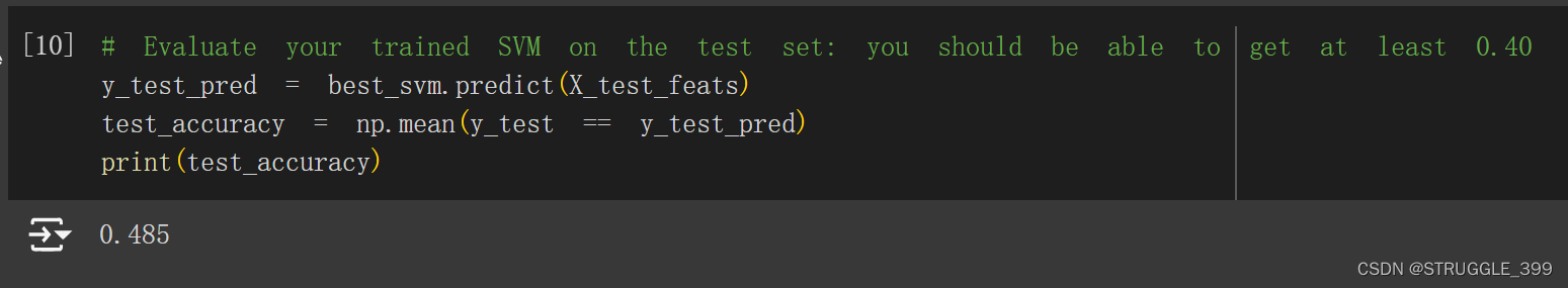
Inline Question 1
下面输出的是一些分类错误的案例,描述你看到的错误分类结果,它们有意义吗?
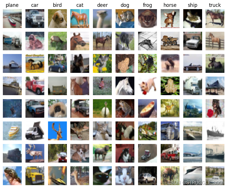
接下来使用两层神经网络基于图像特征进行超参数调整:
from cs231n.classifiers.fc_net import TwoLayerNet
from cs231n.solver import Solver

input_dim = X_train_feats.shape[1]
hidden_dim = 500
num_classes = 10

data = {
    'X_train': X_train_feats,
    'y_train': y_train,
    'X_val': X_val_feats,
    'y_val': y_val,
    'X_test': X_test_feats,
    'y_test': y_test,
}

net = TwoLayerNet(input_dim, hidden_dim, num_classes)
best_net = None

################################################################################
# TODO: Train a two-layer neural network on image features. You may want to    #
# cross-validate various parameters as in previous sections. Store your best   #
# model in the best_net variable.                                              #
################################################################################
# *****START OF YOUR CODE (DO NOT DELETE/MODIFY THIS LINE)*****

best_val = -1
learning_rates = [1e-4, 3e-4, 1e-3, 3e-3, 1e-2, 3e-2, 1e-1]
regularization_strengths = [1e-6, 1e-5, 1e-4, 1e-3, 1e-2, 1e-1, 0, 1]

for lr in learning_rates:
  for reg in regularization_strengths:
    print('learning rate=%f, regularization strength=%f' % (lr, reg))
    net = TwoLayerNet(input_dim, hidden_dim, num_classes, reg=reg)
    solver = Solver(net, data, optim_config={'learning_rate': lr}, num_epochs=10)
    solver.train()
    if best_val < solver.best_val_acc:
      best_net = net
      best_val = solver.best_val_acc
      best_params = (lr, reg)

print('best learning rate=%f, best regularization strength=%f' % best_params)
print('best validation accuracy achieved: %f' % best_val)

# *****END OF YOUR CODE (DO NOT DELETE/MODIFY THIS LINE)*****
最终得到的最好验证精度为 61.1%,对应的超参数组合为:learing rate, regularization strength= (0.100000, 0.000001):
best learning rate=0.100000, best regularization strength=0.000001
best validation accuracy achieved: 0.611000
最终得到的验证精度为 58.9%
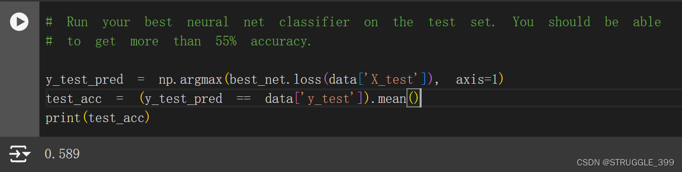


 2026
2026

 被折叠的 条评论
为什么被折叠?
被折叠的 条评论
为什么被折叠?
 到【灌水乐园】发言


