Fisher 线性判别分析及代码实现

原创已于 2023-10-08 18:54:10 修改 · 3.9k 阅读

35 ·

CC 4.0 BY-SA版权

文章标签：

#算法 #python

于 2023-10-08 18:50:12 首次发布

本文介绍了Fisher线性判别分析的基本原理，包括判别函数、投影准则、求解过程，以及如何通过Python实现一个分类实例。文章详细展示了如何计算权向量和分割阈值，并给出了一个具体的代码实现和应用案例。

摘要生成于 C知道，由 DeepSeek-R1 满血版支持，前往体验 >

一、基本原理

1、线性分类器

线性分类器的判别函数为 $g(x)=w^{^{T}}x+w_{0}$ ，其中 $w$ 为一个 n 维列向量，称为权向量或权重； $w_{0}$ 为一个常数，称为阈值权或偏置。

$x = \begin{pmatrix} x_{1}\\ x_{2}\\ ....\\ x_{n}\end{pmatrix}; w = \begin{pmatrix} w_{1}\\ w_{2}\\ ....\\ w_{n}\end{pmatrix}$

2、Fisher线性判别分析

2.1、Fisher线性判别分析的原理

Fisher线性判别分析（Fisher Linear Discriminant Analysis）就是为了求解上述判别函数 $g(x)=w^{^{T}}x+w_{0}$ 中的最优 $w^{*}$ 和 $w_{0}$ ，该方法是利用降维的思想将所有样本点投影到一条直线上，然后选择一个阈值将两类分开（以二分类问题为例），具体如下图所示。

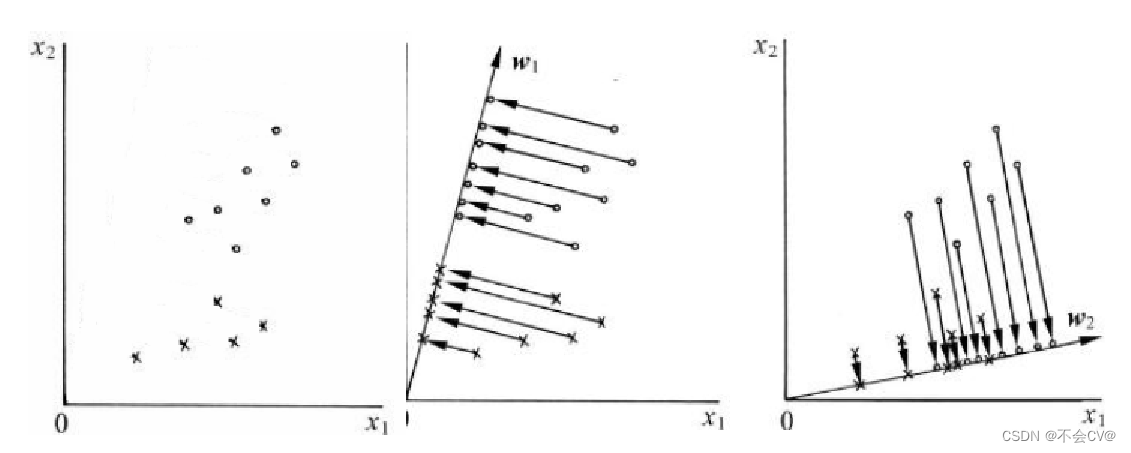
投影的准则： （1）两类之间的距离尽可能远；（2）每一类自身尽可能紧凑。根据上述准则可知图(b)的投影效果图(c)要好。

2.2、求解过程：

2.2.1、权向量求解

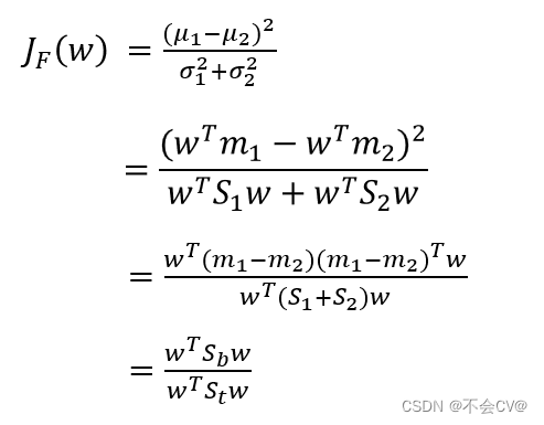
以二分类问题为例，现做出如下约定： $m_{1}$ 和 $m_{2}$ 分别两类（原始）数据的均值向量； $S_{1}$ 和 $S_{2}$ 分别表示两类（原始）数据的离散度矩阵； $\mu _{1}$ 和 $\mu _{2}$ 分别表示两类（投影后，一维）数据的均值； $\sigma _{1}$ 和 $\sigma_{2}$ 分别表示两类（投影后，一维）数据的离散度。则上述投影准则中，准则（1）可以用 $(\mu_{1}-\mu_{2})^{2}$ 越大越好来表示，准则（2）用 $\sigma_{1}^{2} + \sigma_{2}^{2}$ 越小越好来表示。所以Fisher准则函数可用如下的式子来表示：

$J_{F}(w)=\frac{(\mu_{1}-\mu_{2})^{2}}{\sigma_{1}^{2} + \sigma_{2}^{2}}$

此时，优化的目标就变成了下式：

$w_{opt} =argmaxJ_{F}(w)$

定义：（1）类间散度矩阵（给出两种计算方式）

$S_{b} = (m_1-m_2)(m_1-m_2)^{T}$

$S_{b} = P(w_1)P(w_2)(m_1-m_2)(m_1-m_2)^{T}$

（2）类内散度矩阵

$S_{i} =\sum [(x_j-m_i)(x_j-m_i)^{T}]$

（3）总类内散度矩阵（给出两种计算方式）

$S_t=S_1+S_2$

$S_t=P(w_1)S_1+P(w_2)S_2$

则上述的Fisher准则函数可简化为：

最后求解可得： $w^*=S_t^{-1}(m_1-m_2)$

2.2.2、分割阈值求解

分割阈值 $w_0$ 的求解有两种方法：

（1）取投影后两类均值的中点作为分割阈值

$w_0 = -\frac{1}{2}(\mu_1+\mu_2)$

（2）如果投影到一维空间后样本接近正态分布，可以根据样本拟合正态分布，估计分类阈值。

$w_0 = -\frac{1}{2}(m_1+m_2)^TS_t^{-1}(m_1-m_2)-ln\frac{P(w_2)}{P(w_1)}$

3、具体实例

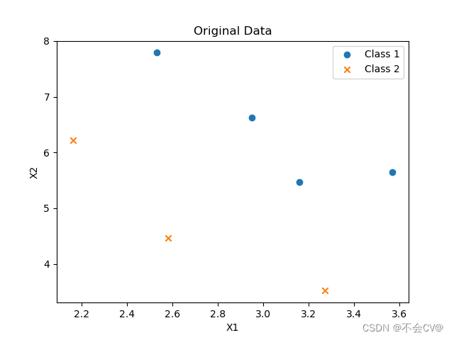
已知样本点及其label如下，要求使用Fisher分类器对其进行分类，并自己设计一个测试集进行测试。

x = np.array([[2.9500, 6.6300], [2.5300, 7.7900],
              [3.5700, 5.6500], [3.1600, 5.4700],
              [2.5800, 4.4600], [2.1600, 6.2200],
              [3.2700, 3.5200]])
label = np.array([1, 1, 1, 1, 2, 2, 2])

原始数据：

测试集：

test = np.array([[5.2500, 4.6500], [5.6400, 2.5300],
                 [2.2400, 2.4500], [3.2100, 2.1800],
                 [5.4500, 5.6700], [1.2800, 2.2200]])

分类结果：

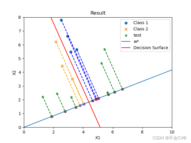
测试集的label预测结果：

二、代码实现

import numpy as np
import matplotlib.pyplot as plt
import math


def calculate_data(x):
    """统计量计算"""
    mean_w = np.mean(x, axis=0)
    scatter_matrix = np.zeros((x.shape[1], x.shape[1]))
    for data in x:
        data = data.reshape((-1, 1))
        mean_w = mean_w.reshape((-1, 1))
        scatter_matrix += (data - mean_w).dot((data - mean_w).T)
    return mean_w, scatter_matrix


def predict(x, w, threshold):
    """标签预测"""
    predict_label = []
    for data in x:
        value = w.T.dot(data) + threshold
        if value > 0:
            predict_label.append(1)
        else:
            predict_label.append(2)
    return predict_label


def subpoint_draw(x, w, color):
    """绘制投影点和投影线"""
    subpoints = np.dot(x, w) / np.dot(w.T, w) * w.T
    plt.scatter(subpoints[:, 0], subpoints[:, 1])
    for i in range(x.shape[0]):
        x_i = x[i]
        subpoint_i = subpoints[i]
        plt.plot([x_i[0], subpoint_i[0]], [x_i[1], subpoint_i[1]],
                 linestyle='--', color=color)


x = np.array([[2.9500, 6.6300], [2.5300, 7.7900],
              [3.5700, 5.6500], [3.1600, 5.4700],
              [2.5800, 4.4600], [2.1600, 6.2200],
              [3.2700, 3.5200]])
label = np.array([1, 1, 1, 1, 2, 2, 2])
test = np.array([[5.2500, 4.6500], [5.6400, 2.5300],
                 [2.2400, 2.4500], [3.2100, 2.1800],
                 [5.4500, 5.6700], [1.2800, 2.2200]])

mu1, s1 = calculate_data(x[label == 1])
mu2, s2 = calculate_data(x[label == 2])

# 计算先验概率
p_p1 = len(x[label == 1]) / len(label)
p_p2 = 1 - p_p1

# 计算s_w和s_b
s_w = p_p1 * s1 + p_p2 * s2
s_b = p_p1 * p_p2 * (mu1 - mu2).dot((mu1 - mu2).T)

# 计算最优解w(投影向量)
w = np.linalg.inv(s_w).dot(mu1 - mu2)

projected_data = test.dot(w)

# 设置决策阈值
threshold = -0.5 * \
    (mu1 + mu2).T.dot(np.linalg.inv(s_w).dot(mu1 - mu2)) - math.log(p_p2 / p_p1)

# 预测测试数据集的标签
predict_label = predict(test, w, threshold)
print(predict_label)

class_1 = x[label == 1]
class_2 = x[label == 2]

# 计算决策面参数
k = 0 - w[0, 0] / w[1, 0]
b = 0 - threshold[0] / w[1, 0]
data = np.linspace(0, 8, 100)
y = k * data + b

# 添加坐标轴标签
plt.xlabel('X1')
plt.ylabel('X2')
# 确定坐标轴范围
plt.xlim(0, 10)
plt.ylim(0, 8)
# 绘制数据分布
plt.scatter(class_1[:, 0], class_1[:, 1], label='Class 1', marker='o')
plt.scatter(class_2[:, 0], class_2[:, 1], label='Class 2', marker='x')
plt.scatter(test[:, 0], test[:, 1], label='test', marker='*')

# 绘制投影方向w*
plt.plot([0, w[0, 0]], [0, w[1, 0]], label='w*')

# 绘制决策面
plt.plot(data, y, label='Decision Surface', color='red')

# 绘制投影点
subpoint_draw(x[label == 1], w, color='blue')
subpoint_draw(x[label == 2], w, color='orange')
subpoint_draw(test, w, color='green')
plt.title('Result')
plt.legend()
plt.show()