笔记：计算机视觉与深度学习-简单的实现一个网络-番外篇

本文链接：https://blog.youkuaiyun.com/weixin_45562510/article/details/115859108

写在开头

1.课程来源及所有代码来源，后面不再每一步中标明了：pytorch官方网站的Tutorials.和Docs.
2.笔记目的：个人学习+增强记忆+方便回顾
3.时间：2021年4月19日
4.同类笔记链接：（钩子：会逐渐增加20210428）
第一讲.第二讲.第三讲.第四讲.第五讲.第六讲.第七讲.第八讲.第九讲.第十讲.第十一讲.番外篇一个简单实现.第十二讲.第十三讲.第十四讲完结.
5.之所以要在基本学习了机器学习课程一周后加入动手的一节，是因为单纯的学习知识是枯燥的，必须要动手做出一个无论大小无论是否有用的东西才能形成正向的反馈。在枯燥学习-奖励性质的正向反馈，如此循环中此有动力激励自己不断学习。思想来源陈云在知乎上的回答.
6.注意符号 SS：意味着我的个人理解，非单纯授课内容，有可能有误哦。

—以下正文—

一、Tutorials

（一）页面介绍

在这里插入图片描述

1.蓝色网站导航、红色tutorials导航、绿色内容。
2.红色导航内区分不同板块，有评价区、学习基本区（这是我们要看的）、训练图像和视频识别区、NLP区、reinforcement learning区等等。但这都是tutorial。

（二）learn the basics

1.使用开源图集MNIST，分类：T恤、…等一堆衣服。
2.辅导课的代码在哪里跑？推荐在云端跑。Each section has a Colab link at the top。如果要在本地跑代码，需要先行安装pytorch，网站提供的安装导引链接.
3.如何使用这份导引？这里有两个分支，有一定熟悉的，使用快速开始。不熟悉的有基础知识的学习导引。

（三）tensor

1.tensor张量，一种类似于数列和矩阵的结构。一种类似于numpy包里ndarrays的数据结构。是pytorch的核心。
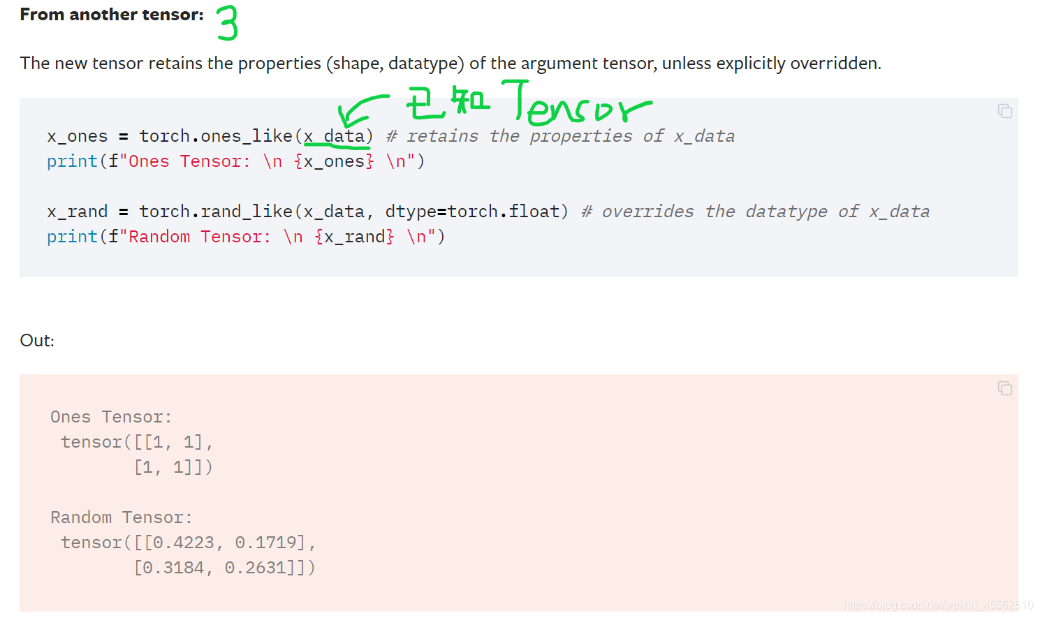
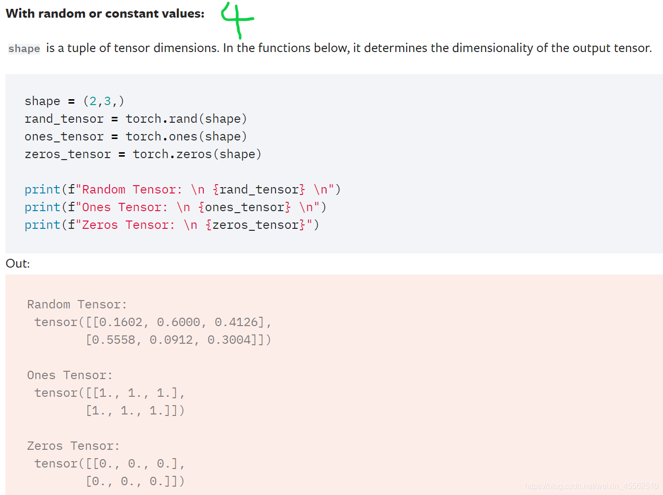
2.tensor的初始化：用直接用矩阵初始化、用numpy array初始化、用另一个tensor初始化（存在完全复制形式，和只使用原tensor的shape，数据和数据格式可以另行命名形式）、通过随机变量或常量初始化。
3.tensor的属性（Attribute）：tensor.shape、tensor.dtype、tensor.device。
4.关于tensor的方法有上百种，有算术的、线性代数的、矩阵复杂操作（切片、索引等等）。通常在GPU上运算比在CPU上更快。通常tensor在CPU上创建，通过.to方法移动到GPU上运算，因此时刻谨记复杂的tensor会导致很大的开销。

# We move our tensor to the GPU if available
if torch.cuda.is_available():
  tensor = tensor.to('cuda')

5.与numpy相同的索引和切片方式
- 输入：

tensor = torch.ones(4, 4)
print('First row: ',tensor[0])
print('First column: ', tensor[:, 0])
print('Last column:', tensor[..., -1])
tensor[:,1] = 0
print(tensor)

输出：

First row:  tensor([1., 1., 1., 1.])
First column:  tensor([1., 1., 1., 1.])
Last column: tensor([1., 1., 1., 1.])
tensor([[1., 0., 1., 1.],
        [1., 0., 1., 1.],
        [1., 0., 1., 1.],
        [1., 0., 1., 1.]])

6.矩阵的拼接
- 输入：

t1 = torch.cat([tensor, tensor, tensor], dim=1)
print(t1)

输出：

tensor([[1., 0., 1., 1., 1., 0., 1., 1., 1., 0., 1., 1.],
        [1., 0., 1., 1., 1., 0., 1., 1., 1., 0., 1., 1.],
        [1., 0., 1., 1., 1., 0., 1., 1., 1., 0., 1., 1.],
        [1., 0., 1., 1., 1., 0., 1., 1., 1., 0., 1., 1.]])

7.算术运算：
- 输入：

# This computes the matrix multiplication（矩阵乘法） between two tensors. 
# y1, y2, y3 will have the same value
y1 = tensor @ tensor.T  #运算符
y2 = tensor.matmul(tensor.T) #调用tensor实例的方法

y3 = torch.rand_like(tensor)
torch.matmul(tensor, tensor.T, out=y3)  #调用torch内的函数，输出赋值给y3
#ss:容易观察到以上矩阵乘法形式不同，但按照tutorial介绍结果相同。

# This computes the element-wise product. 
# z1, z2, z3 will have the same value
z1 = tensor * tensor
z2 = tensor.mul(tensor)

z3 = torch.rand_like(tensor)
torch.mul(tensor, tensor, out=z3)
# ss：既这里运算的是元素的乘积，不是矩阵乘积

8.提取tensor中的元素
- 输入：

agg = tensor.sum()
agg_item = agg.item()
print(agg_item, type(agg_item))

输出：

agg = tensor.sum()
agg_item = agg.item()
print(agg_item, type(agg_item))

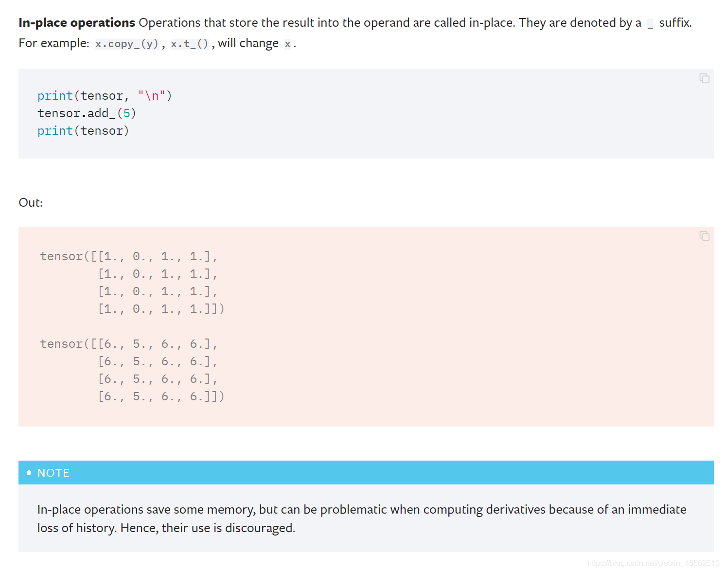
9.in-place操作：我理解为对tensor内元素的操作，很方便但导致导致历史无法回溯。
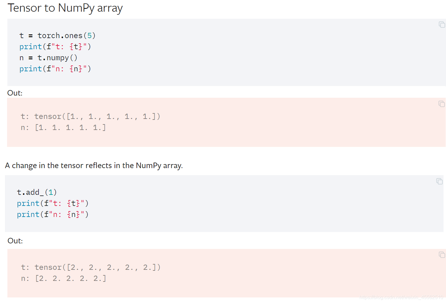
10.与numpy的桥梁（bridge with numpy）
- 10.桥梁，既在创建之后两个对象是相连的，改变tensor也会改变numpy里的对象。（PS:这里的.add就是一个in-place操作）

（四）Datasets & DataLoaders

1.PyTorch provides two data primitives: torch.utils.data.DataLoader and torch.utils.data.Dataset that allow you to use pre-loaded datasets as well as your own data. Dataset stores the samples and their corresponding labels, and DataLoader wraps an iterable(迭代器） around the Dataset to enable easy access to the samples.
2.PyTorch准备了几个数据集用于模型训练的验证，比如MNIST。You can find them here: Image Datasets, Text Datasets, and Audio Datasets
3.载入数据集，有几个参数需要设置，以Fashion MNIST为例：

import torch
from torch.utils.data import Dataset
from torchvision import datasets
from torchvision.transforms import ToTensor, Lambda
import matplotlib.pyplot as plt


training_data = datasets.FashionMNIST(
    root="data",
    train=True,
    download=True,
    transform=ToTensor()
)

test_data = datasets.FashionMNIST(
    root="data",
    train=False,
    download=True,
    transform=ToTensor()
)

4.之后介绍了部分展示数据集、简单的创建自己的数据集，功能现在用不到，不再贴上来，有需要再去看。
5.我们总是希望更细粒度（更小批量）的使用训练数据集，希望每个epoch（可以理解为一轮）都对数据进行洗牌，希望处理速度快。Dataloaders是一个提供简单API的迭代器。
6.以数据集实例为参数，创建Dataloaders实例

from torch.utils.data import DataLoader

train_dataloader = DataLoader(training_data, batch_size=64, shuffle=True)
test_dataloader = DataLoader(test_data, batch_size=64, shuffle=True)

7.迭代（我感觉是逐批访问，不确定？？）通过Dataloaders：通过函数iter和函数next能从实例中获得所有对象，该函数返回features和labels两个实例组，？可用下标逐个访问？。

# Display image and label.
train_features, train_labels = next(iter(train_dataloader))
print(f"Feature batch shape: {train_features.size()}")
print(f"Labels batch shape: {train_labels.size()}")
img = train_features[0].squeeze() #用于输出图片 
label = train_labels[0]
plt.imshow(img, cmap="gray") #用于输出图片 
plt.show() #用于输出图片 
print(f"Label: {label}")
# 中间输出图片略
# 其输出为：
Feature batch shape: torch.Size([64, 1, 28, 28])
Labels batch shape: torch.Size([64])
Label: 2

（五）tansforms（可理解为图像规整成标准形式）

1.数据可能不符合接口标准，用transforms操纵数据使其符合接口。
2.所有TorchVision datasets（既包含我们将要使用的Fashion MNIST数据集和其他测试模型可训练性的数据集）都有两个参数 -transform 调整特征和 target_transform 调整标签。另外torchvision.transforms模块提供几种常用的变换的封装。
3.Fashion MNIST数据集图片是PIL格式，标签为整数。为了训练，我们需要图片转换成标准化张量，标签转换为one-hot编码的张量。为进行这种变换，我们使用orchvision.transforms模块的ToTensor 和 Lambda。

from torchvision import datasets
from torchvision.transforms import ToTensor, Lambda

ds = datasets.FashionMNIST(
    root="data",
    train=True,
    download=True,
    transform=ToTensor(),
    target_transform=Lambda(lambda y: torch.zeros(10, dtype=torch.float).scatter_(0, torch.tensor(y), value=1))
)

6.1ToTensor 把 PIL image 或 NumPy ndarray 变为 FloatTensor. and 将每个像素点的取值范围（一般为0-255）对应到 range [0., 1.]
6.2Lambda transforms 用户定义的lambda函数. 这里, 我们定义了一个函数将整数变为 one-hot编码的 tensor. 它首先创建一个10维张量 (the number of labels in our dataset) and calls scatter_ which assigns a value=1 on the index as given by the label y.（看不懂，先不管了）

（六）建立模型

1.The torch.nn（包） namespace provides all the building blocks you need to build your own neural network.PyTorch中的每一个模型都是the nn.Module的子类。模型中的很多层也是由其他模型组成的，使用nn.Module这样一种网状继承结构方便管理复杂的模型。

import os
import torch
from torch import nn
from torch.utils.data import DataLoader
from torchvision import datasets, transforms

2.先检查GPU是否可用

device = 'cuda' if torch.cuda.is_available() else 'cpu'
print('Using {} device'.format(device))

3.定义一个网络：子类继承自nn.Module，并用__init__初始化，每个nn.Module子类都有一个forward方法用于input数据。

class NeuralNetwork(nn.Module):
    def __init__(self):
        super(NeuralNetwork, self).__init__()
        self.flatten = nn.Flatten()
        self.linear_relu_stack = nn.Sequential(
            nn.Linear(28*28, 512),
            nn.ReLU(),
            nn.Linear(512, 512),
            nn.ReLU(),
            nn.Linear(512, 10),
            nn.ReLU()
        )

    def forward(self, x):
        x = self.flatten(x)
        logits = self.linear_relu_stack(x)
        return logits

4.建立并加载（CPU/GPU）并打印检查一下模型的层数

model = NeuralNetwork().to(device)
print(model)

5.使用该模型，我们将输入数据传递给它。这将执行模型执行forward以及一些后台操作。不要直接调用model.forward()！
在输入上调用模型将返回一个10维张量，其中包含每个类的原始预测值。我们通过将其传递给nn.Softmax模块来获得预测概率。

X = torch.rand(1, 28, 28, device=device)
logits = model(X)
pred_probab = nn.Softmax(dim=1)(logits)
y_pred = pred_probab.argmax(1)
print(f"Predicted class: {y_pred}")

# 输出：
Predicted class: tensor([5], device='cuda:0')

6.之后带着试验性的介绍了几个函数，及其实例。
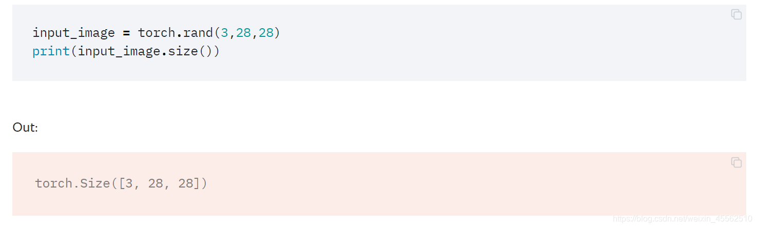
创建32828的张量，命名为input_image。

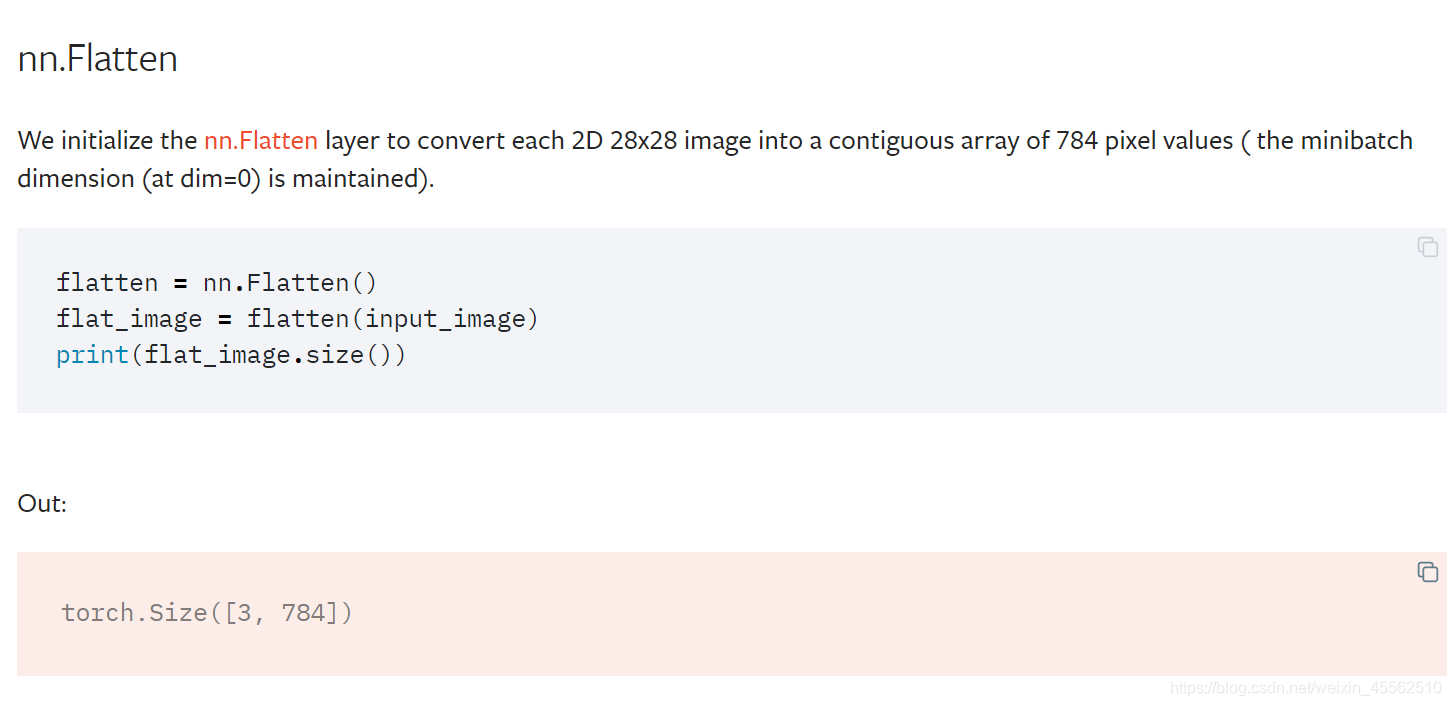
nn.Flatten用于将32828tensor拍平成3784的tensor。（既内部默认定义时后边的2828是用于表示图像X/Y轴的，前面的3是图像张数）

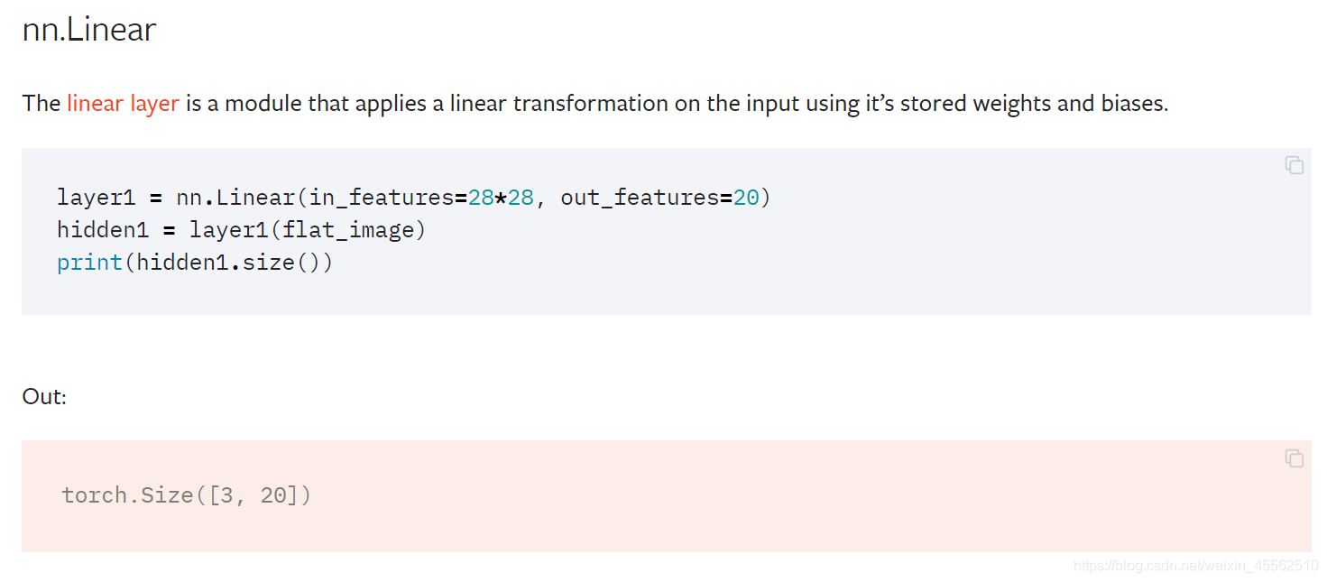
用nn.linear创建线性变换层（卷积层？），将数据变为3*20

创建nn.ReLU层，激活函数。其处理情况和函数如下图所示：

print(f"Before ReLU: {hidden1}\n\n")
hidden1 = nn.ReLU()(hidden1)
print(f"After ReLU: {hidden1}")

上程序段打印结果，既relu的变换前后数组情况：

Before ReLU: tensor([[-0.1086,  0.3614,  0.3995, -0.1273,  0.0947,  0.2789, -0.1394,  0.0904,
          0.2180,  0.0671, -0.1933, -0.2972,  0.1351,  0.3036,  0.3299, -0.3691,
          0.0987, -0.5753, -0.2421,  0.7786],
        [ 0.1127,  0.2443,  0.2404, -0.0956, -0.3439,  0.2791,  0.0406, -0.0495,
          0.1717,  0.0669,  0.1039,  0.1162, -0.1022, -0.1204, -0.1525, -0.1632,
          0.4457, -0.3969, -0.3505,  0.4792],
        [-0.2279,  0.5577,  0.5916,  0.0490, -0.0118,  0.3936,  0.0497, -0.0625,
          0.5442,  0.1243, -0.0236,  0.0471,  0.1432,  0.1569, -0.1530, -0.7931,
          0.1179, -0.1727,  0.0559,  0.4706]], grad_fn=<AddmmBackward>)


After ReLU: tensor([[0.0000, 0.3614, 0.3995, 0.0000, 0.0947, 0.2789, 0.0000, 0.0904, 0.2180,
         0.0671, 0.0000, 0.0000, 0.1351, 0.3036, 0.3299, 0.0000, 0.0987, 0.0000,
         0.0000, 0.7786],
        [0.1127, 0.2443, 0.2404, 0.0000, 0.0000, 0.2791, 0.0406, 0.0000, 0.1717,
         0.0669, 0.1039, 0.1162, 0.0000, 0.0000, 0.0000, 0.0000, 0.4457, 0.0000,
         0.0000, 0.4792],
        [0.0000, 0.5577, 0.5916, 0.0490, 0.0000, 0.3936, 0.0497, 0.0000, 0.5442,
         0.1243, 0.0000, 0.0471, 0.1432, 0.1569, 0.0000, 0.0000, 0.1179, 0.0000,
         0.0559, 0.4706]], grad_fn=<ReluBackward0>)

7.新的类nn.Sequential，nn.Sequential是模块的有序容器。数据按照定义的顺序通过所有模块。可以使用有序容器将类似的快速构件的神经网络组合在一起，不妨命名为seq_modules。

seq_modules = nn.Sequential(
    flatten,
    layer1,
    nn.ReLU(),
    nn.Linear(20, 10)
)
input_image = torch.rand(3,28,28)
logits = seq_modules(input_image)

其中的flatten、layer1是上面实例化过的。

8.新的类nn.Softmax，就是之前课程介绍过的方法，实例化和调用代码如下。

softmax = nn.Softmax(dim=1)
pred_probab = softmax(logits)

（七）TORCH.AUTOGRAD梯度的反向传播

1.损失计算的简单示例
其中的requires_grad=True是一个默认为真标识符，用于标明变量需要梯度计算

import torch

x = torch.ones(5)  # input tensor
y = torch.zeros(3)  # expected output
w = torch.randn(5, 3, requires_grad=True)
b = torch.randn(3, requires_grad=True)
z = torch.matmul(x, w)+b
loss = torch.nn.functional.binary_cross_entropy_with_logits(z, y)

这一function知道正向计算的路径和反向计算的路径，反向传播的存储位置存储在一个张量的grad_fn属性中。

print('Gradient function for z =',z.grad_fn)
print('Gradient function for loss =', loss.grad_fn)
--------------------------------
输出：
Gradient function for z = <AddBackward0 object at 0x7f8cb7938dd8>
Gradient function for loss = <BinaryCrossEntropyWithLogitsBackward object at 0x7f8cb7938dd8>

计算梯度

loss.backward()
print(w.grad)
print(b.grad)
---------------------
输出：
tensor([[0.2863, 0.2387, 0.3316],
        [0.2863, 0.2387, 0.3316],
        [0.2863, 0.2387, 0.3316],
        [0.2863, 0.2387, 0.3316],
        [0.2863, 0.2387, 0.3316]])
tensor([0.2863, 0.2387, 0.3316])

2.不重要的题外话，若不再需要梯度反向传递，通过以下方法：

------------------------------------------
# 方法1
z = torch.matmul(x, w)+b
print(z.requires_grad)

with torch.no_grad():
    z = torch.matmul(x, w)+b
print(z.requires_grad)
------------------------------
输出：
True
False
------------------------------------------
#方法2
z = torch.matmul(x, w)+b
z_det = z.detach()
print(z_det.requires_grad)
-------------------------------
输出：
False

（八）训练

1.收集整理上面提到的可以用于建立模型和加载训练集的代码

import torch
from torch import nn
from torch.utils.data import DataLoader
from torchvision import datasets
from torchvision.transforms import ToTensor, Lambda

training_data = datasets.FashionMNIST(
    root="data",
    train=True,
    download=True,
    transform=ToTensor()
)

test_data = datasets.FashionMNIST(
    root="data",
    train=False,
    download=True,
    transform=ToTensor()
)

train_dataloader = DataLoader(training_data, batch_size=64)
test_dataloader = DataLoader(test_data, batch_size=64)

class NeuralNetwork(nn.Module):
    def __init__(self):
        super(NeuralNetwork, self).__init__()
        self.flatten = nn.Flatten()
        self.linear_relu_stack = nn.Sequential(
            nn.Linear(28*28, 512),
            nn.ReLU(),
            nn.Linear(512, 512),
            nn.ReLU(),
            nn.Linear(512, 10),
            nn.ReLU()
        )

    def forward(self, x):
        x = self.flatten(x)
        logits = self.linear_relu_stack(x)
        return logits

model = NeuralNetwork()

2.设置超参数：学习率、一批数量、epochs。

learning_rate = 1e-3
batch_size = 64
epochs = 5

3.损失函数的计算，常见的损失函数包括用于回归任务的nn.MSELoss（均方误差）和用于分类的nn.NLLLoss（负对数似然）。 nn.CrossEntropyLoss（交叉熵损失）结合nn.LogSoftmax和nn.NLLLoss。

# Initialize the loss function
loss_fn = nn.CrossEntropyLoss()

4.优化器，优化算法定义了该过程的执行方式（在本例中，我们使用随机梯度下降法）。所有优化逻辑都封装在optimizer对象中。在这里，我们使用SGD优化器。此外， PyTorch中提供了许多不同的优化器，例如ADAM和RMSProp，它们对于不同类型的模型和数据更有效。

optimizer = torch.optim.SGD(model.parameters(), lr=learning_rate)

5.整合上面的损失计算和优化器定义，下面进行全面的实施。
首先定义训练函数train_loop和测试函数test_loop

def train_loop(dataloader, model, loss_fn, optimizer):
    size = len(dataloader.dataset)
    for batch, (X, y) in enumerate(dataloader):
        # Compute prediction and loss
        pred = model(X)
        loss = loss_fn(pred, y)

        # Backpropagation
        optimizer.zero_grad()
        loss.backward()
        optimizer.step()

        if batch % 100 == 0:
            loss, current = loss.item(), batch * len(X)
            print(f"loss: {loss:>7f}  [{current:>5d}/{size:>5d}]")


def test_loop(dataloader, model, loss_fn):
    size = len(dataloader.dataset)
    test_loss, correct = 0, 0

    with torch.no_grad():
        for X, y in dataloader:
            pred = model(X)
            test_loss += loss_fn(pred, y).item()
            correct += (pred.argmax(1) == y).type(torch.float).sum().item()

    test_loss /= size
    correct /= size
    print(f"Test Error: \n Accuracy: {(100*correct):>0.1f}%, Avg loss: {test_loss:>8f} \n")

初始化损失函数和优化器，并将其传递给train_loop和test_loop。增加epochs数以跟踪模型的改进性能。

loss_fn = nn.CrossEntropyLoss()
optimizer = torch.optim.SGD(model.parameters(), lr=learning_rate)

epochs = 10
for t in range(epochs):
    print(f"Epoch {t+1}\n-------------------------------")
    train_loop(train_dataloader, model, loss_fn, optimizer)
    test_loop(test_dataloader, model, loss_fn)
print("Done!")

最终输出：

Epoch 1
-------------------------------
loss: 2.289717  [    0/60000]
loss: 2.287769  [ 6400/60000]
loss: 2.271825  [12800/60000]
loss: 2.270507  [19200/60000]
loss: 2.258810  [25600/60000]
loss: 2.226384  [32000/60000]
loss: 2.238326  [38400/60000]
loss: 2.208152  [44800/60000]
loss: 2.207475  [51200/60000]
loss: 2.179998  [57600/60000]
Test Error:
 Accuracy: 52.3%, Avg loss: 0.034431
 
#由于太长，我删去了 2-9 epochs的显示

Epoch 10
-------------------------------
loss: 1.177898  [    0/60000]
loss: 1.337143  [ 6400/60000]
loss: 1.155820  [12800/60000]
loss: 1.373691  [19200/60000]
loss: 1.142431  [25600/60000]
loss: 1.066248  [32000/60000]
loss: 1.183711  [38400/60000]
loss: 1.043591  [44800/60000]
loss: 1.105449  [51200/60000]
loss: 1.146227  [57600/60000]
Test Error:
 Accuracy: 60.4%, Avg loss: 0.018788

Done!

（九）保存、加载并使用模型

1.保存代码如下

torch.save(model.state_dict(), "model.pth")

2.加载代码如下

model = NeuralNetwork()
model.load_state_dict(torch.load("model.pth"))

3.从测试集中随机抽取一张用于预测

classes = [
    "T-shirt/top",
    "Trouser",
    "Pullover",
    "Dress",
    "Coat",
    "Sandal",
    "Shirt",
    "Sneaker",
    "Bag",
    "Ankle boot",
]

model.eval()
x, y = test_data[0][0], test_data[0][1]
with torch.no_grad():
    pred = model(x)
    predicted, actual = classes[pred[0].argmax(0)], classes[y]
    print(f'Predicted: "{predicted}", Actual: "{actual}"')