sklearn 主成分分析法 PCA和IPCA

主成分分析法 (PCA) 是一种常用的数据分析手段。对于一组不同维度 之间可能存在线性相关关系的数据，PCA 能够把这组数据通过正交变换变 成各个维度之间线性无关的数据。经过 PCA 处理的数据中的各个样本之间 的关系往往更直观，所以它是一种非常常用的数据分析和预处理工具。PCA处理之后的数据各个维度之间是线性无关的，通过剔除方差较小的那些维度上的数据我们可以达到数据降维的目的。

将原 先的n个特征用数目更少的m个特征取代，新特征是旧特征的线性组合，这些线性组合最大化样本 方差，从而保留样本尽可能多的信息，并且m个特征互不相关。

用几何观点来看，PCA主成分分析方法可以看成通过正交变换，对坐标系进行旋转和平移，并保留 样本点投影坐标方差最大的前几个新的坐标。

通过PCA主成分分析，可以帮助去除样本中的噪声信息，便于进一步做回归分析。

import matplotlib.pyplot as plt
from mpl_toolkits.mplot3d import Axes3D
from sklearn import datasets
from sklearn.decomposition import PCA

# import some data to play with
iris = datasets.load_iris()
# 使用前两个特征
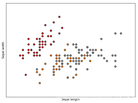
X = iris.data[:, :2]  # we only take the first two features.
y = iris.target
# 得到
x_min, x_max = X[:, 0].min() - .5, X[:, 0].max() + .5
y_min, y_max = X[:, 1].min() - .5, X[:, 1].max() + .5

plt.figure(2, figsize=(8, 6))
# 清屏
plt.clf()

# Plot the training points
plt.scatter(X[:, 0], X[:, 1], c=y, cmap=plt.cm.Set1,
            edgecolor='k')
plt.xlabel('Sepal length')
plt.ylabel('Sepal width')

plt.xlim(x_min, x_max)
plt.ylim(y_min, y_max)
plt.xticks(())
plt.yticks(())

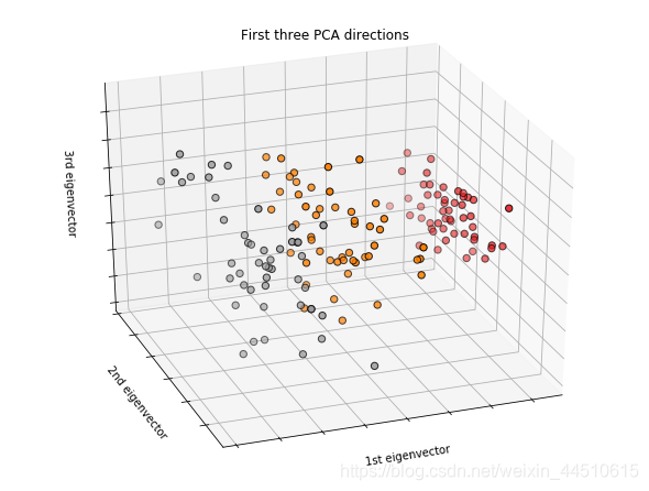
#因为iris4个特征，降维到3个来绘制3D图

#绘制前三个PCA尺寸 新建画布
fig = plt.figure(1, figsize=(8, 6))
ax = Axes3D(fig, elev=-150, azim=110)
# 将前三个特征作为桑坐标轴
X_reduced = PCA(n_components=3).fit_transform(iris.data)
ax.scatter(X_reduced[:, 0], X_reduced[:, 1], X_reduced[:, 2], c=y,
           cmap=plt.cm.Set1, edgecolor='k', s=40)

ax.set_title("First three PCA directions")
ax.set_xlabel("1st eigenvector")
ax.w_xaxis.set_ticklabels([])
ax.set_ylabel("2nd eigenvector")
ax.w_yaxis.set_ticklabels([])
ax.set_zlabel("3rd eigenvector")
ax.w_zaxis.set_ticklabels([])

plt.show()

import numpy as np
import matplotlib.pyplot as plt
from mpl_toolkits.mplot3d import Axes3D

# PCA
from sklearn import decomposition
from sklearn import datasets

np.random.seed(5)

centers = [[1, 1], [-1, -1], [1, -1]]
iris = datasets.load_iris()
X = iris.data
y = iris.target

fig = plt.figure(1, figsize=(4, 3))
plt.clf()

ax = Axes3D(fig, rect=[0, 0, .95, 1], elev=48, azim=134)

plt.cla()
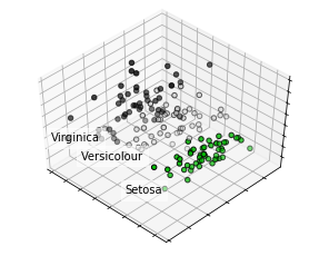
pca = decomposition.PCA(n_components=3)
pca.fit(X)
X = pca.transform(X)
# 分类
for name, label in [('Setosa', 0), ('Versicolour', 1), ('Virginica', 2)]:
    ax.text3D(X[y == label, 0].mean(),
              X[y == label, 1].mean() + 1.5,
              X[y == label, 2].mean(), name,
              horizontalalignment='center',
              bbox=dict(alpha=.5, edgecolor='w', facecolor='w'))
# Reorder the labels to have colors matching the cluster results
y = np.choose(y, [1, 2, 0]).astype(np.float)
ax.scatter(X[:, 0], X[:, 1], X[:, 2], c=y, cmap=plt.cm.nipy_spectral,
           edgecolor='k')

ax.w_xaxis.set_ticklabels([])
ax.w_yaxis.set_ticklabels([])
ax.w_zaxis.set_ticklabels([])

plt.show()

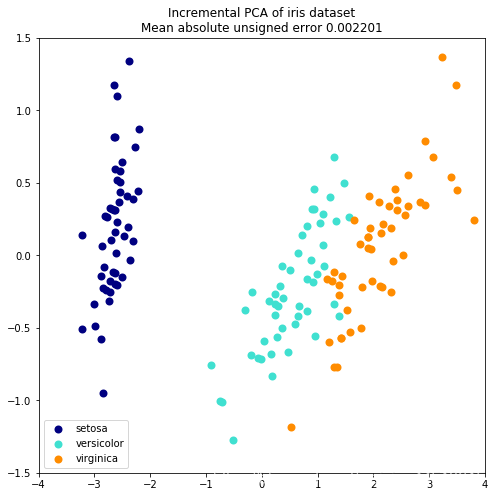
超大规模数据降维Incremental PCA

当要分解的数据集太大而无法放入内存时，增量主成分分析（IPCA）通常用作主成分分析（PCA）的替代。

也就是将数据分成更少的特征维度

import numpy as np
import matplotlib.pyplot as plt

from sklearn.datasets import load_iris
# 导入IPCA
from sklearn.decomposition import PCA, IncrementalPCA

iris = load_iris()
X = iris.data
y = iris.target

# 分成2份 
n_components = 2
# 使用ipca
ipca = IncrementalPCA(n_components=n_components, batch_size=10)
X_ipca = ipca.fit_transform(X)
# 使用pca

pca = PCA(n_components=n_components)
X_pca = pca.fit_transform(X)

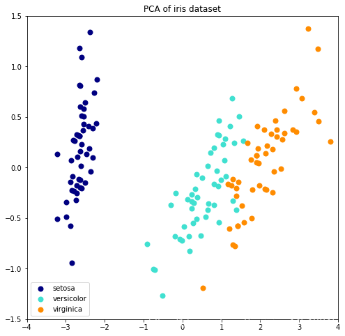
colors = ['navy', 'turquoise', 'darkorange']

for X_transformed, title in [(X_ipca, "Incremental PCA"), (X_pca, "PCA")]:
    plt.figure(figsize=(8, 8))
    for color, i, target_name in zip(colors, [0, 1, 2], iris.target_names):
        plt.scatter(X_transformed[y == i, 0], X_transformed[y == i, 1],
                    color=color, lw=2, label=target_name)

    if "Incremental" in title:
        err = np.abs(np.abs(X_pca) - np.abs(X_ipca)).mean()
        plt.title(title + " of iris dataset\nMean absolute unsigned error "
                  "%.6f" % err)
    else:
        plt.title(title + " of iris dataset")
    plt.legend(loc="best", shadow=False, scatterpoints=1)
    plt.axis([-4, 4, -1.5, 1.5])

plt.show()

参考：https://scikit-learn.org/stable/index.html#