Classification 分类学习

声明

来源于莫烦Python：Classification 分类学习

---

分类问题的通俗理解

 分类和回归在于输出变量的类型上。通俗来讲，连续变量预测，如预测房价问题，属于回归问题; 离散变量预测，如把东西分成几类，属于分类问题。

---

代码

import tensorflow as tf
from tensorflow.examples.tutorials.mnist import input_data
# number 1 to 10 data
mnist = input_data.read_data_sets('MNIST_data', one_hot=True)

def add_layer(inputs, in_size, out_size, activation_function=None,):
    # add one more layer and return the output of this layer
    Weights = tf.Variable(tf.random_normal([in_size, out_size]))
    biases = tf.Variable(tf.zeros([1, out_size]) + 0.1,)
    Wx_plus_b = tf.matmul(inputs, Weights) + biases
    if activation_function is None:
        outputs = Wx_plus_b
    else:
        outputs = activation_function(Wx_plus_b,)
    return outputs

def compute_accuracy(v_xs, v_ys):
    global prediction
    y_pre = sess.run(prediction, feed_dict={xs: v_xs})
    correct_prediction = tf.equal(tf.argmax(y_pre,1), tf.argmax(v_ys,1))
    accuracy = tf.reduce_mean(tf.cast(correct_prediction, tf.float32))
    result = sess.run(accuracy, feed_dict={xs: v_xs, ys: v_ys})
    return result

# define placeholder for inputs to network
xs = tf.placeholder(tf.float32, [None, 784]) # 28x28
ys = tf.placeholder(tf.float32, [None, 10])

# add output layer
prediction = add_layer(xs, 784, 10,  activation_function=tf.nn.softmax)

# the error between prediction and real data
cross_entropy = tf.reduce_mean(-tf.reduce_sum(ys * tf.log(prediction),
                                              reduction_indices=[1]))       # loss
train_step = tf.train.GradientDescentOptimizer(0.5).minimize(cross_entropy)

sess = tf.Session()
init = tf.global_variables_initializer()
sess.run(init)

for i in range(1000):
    batch_xs, batch_ys = mnist.train.next_batch(100)  # 分批进行学习，时间短，效果不一定比整套的差
    sess.run(train_step, feed_dict={xs: batch_xs, ys: batch_ys})
    if i % 50 == 0:
        print(compute_accuracy(
            mnist.test.images, mnist.test.labels))

---

代码释义

1. MNIST 数据

首先准备数据（MNIST库）

from tensorflow.examples.tutorials.mnist import input_data
mnist = input_data.read_data_sets('MNIST_data', one_hot=True)

MNIST库是手写体数字库，差不多是这样子的

数据中包含55000张训练图片，每张图片的分辨率是28×28，所以我们的训练网络输入应该是28×28=784个像素数据。

搭建网络

xs = tf.placeholder(tf.float32, [None, 784]) # 28x28

每张图片都表示一个数字，所以我们的输出是数字0到9，共10类。

ys = tf.placeholder(tf.float32, [None, 10])

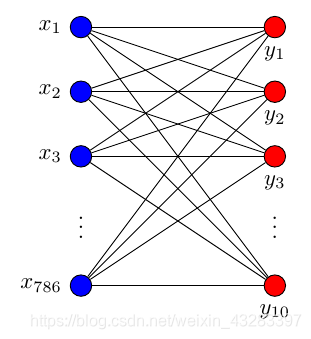
调用add_layer函数搭建一个最简单的训练网络结构，只有输入层和输出层。

prediction = add_layer(xs, 784, 10, activation_function=tf.nn.softmax)

其中输入数据是784个特征，输出数据是10个特征，激励采用softmax函数，网络结构图是这样子的

2. Cross entropy loss

loss函数（即最优化目标函数）选用交叉熵函数。交叉熵用来衡量预测值和真实值的相似程度，如果完全相同，它们的交叉熵等于零。

cross_entropy = tf.reduce_mean(-tf.reduce_sum(ys * tf.log(prediction),
reduction_indices=[1])) # loss

train方法（最优化算法）采用梯度下降法。

train_step = tf.train.GradientDescentOptimizer(0.5).minimize(cross_entropy)
sess = tf.Session()
init = tf.global_variables_initializer()
sess.run(init)
sess.run(tf.global_variables_initializer())

3. 训练

现在开始train，每次只取100张图片，免得数据太多训练太慢。

batch_xs, batch_ys = mnist.train.next_batch(100)
sess.run(train_step, feed_dict={xs: batch_xs, ys: batch_ys})

每训练50次输出一下预测精度

if i % 50 == 0:
        print(compute_accuracy(
            mnist.test.images, mnist.test.labels))

输出结果如下：

0.1615
0.665
0.7495
0.7905
0.808
0.8262
0.8359
0.8432
0.8486
0.8538
0.8579
0.8592
0.8619
0.8613
0.8645
0.8658
0.8702
0.8719
0.8734
0.8754