NonLinear Regression Problem & Ridge Regression

最新推荐文章于 2024-11-09 16:57:04 发布

原创

最新推荐文章于 2024-11-09 16:57:04 发布 · 775 阅读

1 ·

CC 4.0 BY-SA版权

文章标签：

#Python #Numpy #sklearn #机器学习

本文通过非线性回归问题引入，探讨如何使用线性回归在特征空间中逼近复杂函数，通过创建非线性回归问题并进行岭回归分析。通过网格搜索找到最佳正则化参数，并可视化结果对比了OLS、岭回归与目标函数的表现。

摘要生成于 C知道，由 DeepSeek-R1 满血版支持，前往体验 >

Part One : Basis for Nonlinear Regression

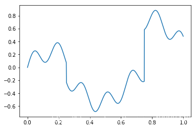
In this part we’re going to investigate how to use linear regression to approximate and estimate complicated functions. For example, suppose we want to fit the following function on the interval [0,1] :

Import Modules

import numpy as np
import matplotlib.pyplot as plt
import pandas as pd

Create a problem

def y(x):
    ret = .15*np.sin(40*x) 
    ret = ret + .25*np.sin(10*x)
    step_fn1 = np.zeros(len(x))
    step_fn1[x >= .25] = 1
    step_fn2 = np.zeros(len(x))
    step_fn2[x >= .75] = 1
    ret = ret - 0.3*step_fn1 + 0.8 *step_fn2 
    return ret

x = np.arange(0.0, 1.0, 0.001)
plt.plot(x, y(x))
plt.show()

在这里插入图片描述

Plot the graph and see the functions

Here the input space, shown on the x-axis, is very simple – it’s just the interval $[0, 1]$ . The output space is reals ( $R\mathcal{R}$ ), and a graph of the function $(x,y(x))∣x∈[0,1]}\{(x,y(x)) \mid x \in [0,1]\}$ is shown above. Clearly a linear function of the input will not give a good approximation to the function. There are many ways to construct nonlinear functions of the input. Some popular approaches in machine learning are regression trees, neural networks, and local regression (e.g. LOESS). However, our approach here will be to map the input space $[0, 1]$ into a “feature space” $Rd\mathcal{R}^d$ , and then run standard linear regression in the feature space.

Feature extraction, or “featurization”, maps an input from some input space $X\mathcal{X}$ to a vector in $Rd\mathcal{R}^d$ . Here our input space is $X=[0,1]\mathcal{X}=[0,1]$ , so we could write our feature mapping as a function $Φ:[0,1]→Rd\Phi:[0,1]\to\mathcal{R}^d$ . The vector $Φ(x)\Phi(x)$ is called a feature vector, and each entry of the vector is called a feature. Our feature mapping is typically defined in terms of a set of functions, each computing a single entry of the feature vector. For example, let’s define a feature function $ϕ1(x)=1(x≥0.25)\phi_1(x)=1(x\ge0.25)$ . The $1(⋅)1(\cdot)$ denotes an indicator function, which is 1 if the expression in the parenthesis is true, and 0 otherwise. So $ϕ1(x)\phi_1(x)$ is $1$ if $x≥0.25x\ge0.25$ and $0$ otherwise. This function produces a “feature” of x. Let’s define two more features: $ϕ2(x)=1(x≥0.5)\phi_2(x)=1(x\ge0.5)$ and $ϕ3(x)=1(x≥0.75)\phi_3(x)=1(x\ge0.75)$ . Now we can define a feature mapping into $R3\mathcal{R}^3$ as:
$\Phi(x) = ( \phi_1(x), \phi_2(x), \phi_3(x) ).$

Let’s code up these feature functions explicitly and plot them as functions of $x$ :

def step_fn_generator(step_loc=0):
    def f(x):
        ret = np.zeros(len(x))
        ret[x >= step_loc] = 1
        return ret
    return f

phi_1 = step_fn_generator(0.25)
phi_2 = step_fn_generator(0.50)
phi_3 = step_fn_generator(0.75)

x = np.arange(0.0