Week One : Gradient Decent & SGD

Week One : Linear Regression & Risk Minimization

Preparation I : Import Modules

import sys
import numpy as np
import pandas as pd
import matplotlib.pyplot as plt
from sklearn.model_selection import train_test_split

Preparation II : Import dataset

data = np.loadtxt("data.csv" , skiprows=1, delimiter = ',')

Preparing III : Split dataset -> (Train , Test)

data_train , data_test = train_test_split(data , shuffle = False)
data_train, data_test

(array([[ 0.        ,  0.        ,  0.        , ..., -0.7818242 ,
         -3.909121  , -1.37657523],
        [ 0.        ,  0.        ,  0.        , ..., -0.77870504,
         -3.89352522,  0.87878245],
        [ 0.        ,  0.        ,  0.        , ..., -0.77755137,
         -3.88775684,  1.10870068],
        ...,
        [ 1.        ,  1.        ,  1.        , ..., -0.2263517 ,
         -1.13175852, -2.25509181],
        [ 1.        ,  1.        ,  1.        , ..., -0.22509951,
         -1.12549756, -2.5520492 ],
        [ 1.        ,  1.        ,  1.        , ..., -0.22101106,
         -1.10505529, -4.44969556]]),
 array([[ 1.00000000e+00,  1.00000000e+00,  1.00000000e+00, ...,
         -2.15876877e-01, -1.07938439e+00, -4.51006402e+00],
        [ 1.00000000e+00,  1.00000000e+00,  1.00000000e+00, ...,
         -2.14082461e-01, -1.07041230e+00, -4.06896259e+00],
        [ 1.00000000e+00,  1.00000000e+00,  1.00000000e+00, ...,
         -2.12904582e-01, -1.06452291e+00, -3.37386281e+00],
        ...,
        [ 1.00000000e+00,  1.00000000e+00,  1.00000000e+00, ...,
         -5.08916428e-03, -2.54458214e-02,  3.37935567e+00],
        [ 1.00000000e+00,  1.00000000e+00,  1.00000000e+00, ...,
         -3.21856040e-03, -1.60928020e-02,  2.46885009e+00],
        [ 1.00000000e+00,  1.00000000e+00,  1.00000000e+00, ...,
         -1.82913081e-03, -9.14565404e-03,  3.96120935e+00]]))

x_train , y_train = np.split(data_train,[-1],1)
x_test , y_test = np.split(data_train,[-1],1)

Part One : Feature Normalization

Function : def feature_normalization(train, test)

Description: Rescale the data so that each feature in the training set is in the interval [0,1], and apply the same transformations to the test set, using the statistics computed on the training set.

Args:
    train - training set, a 2D numpy array of size (num_instances, num_features)
    test - test set, a 2D numpy array of size (num_instances, num_features)

Returns:
    train_normalized - training set after normalization
    test_normalized - test set after normalization

def feature_normalization(train , test) :
    train = train.T   # Transform dataset so that we can use the column data
    for i in range(len(train)) :  #for loop normalization one by one
        Max = max(train[i])
        Min = min(train[i])
        if Max > Min :    #To find out if the variable is constant. 
            for j in range(len(train[i])) :
                train[i,j] = (train[i,j] - Min) / (Max - Min)    #Normalization
    test = test.T
    for i in range(len(test)) :
        Max = max(test[i])
        Min = min(test[i])
        if Max > Min :
            for j in range(len(test[i])) :
                test[i,j] = (test[i,j] - Min) / (Max - Min)
    return train.T , test.T  #Return the result

x_train , x_test = feature_normalization(x_train , x_test)
y_train , y_test = feature_normalization(y_train , y_test)
y_train = y_train.squeeze()
y_test = y_train.squeeze()

Part Two : Gradient Descent Setup

In linear regression, we consider the hypothesis space of linear functions
$h_{\theta }:R^d\to R$, where
$$h_{\theta }(x)={\theta }^{T}x,$$
for $\theta ,x\in R^d$, and we choose $\theta$ that minimizes
the following ``average square loss’’ objective function:
$$J(\theta )=\frac{1}{m}\sum _{i=1}^m{\left(h_{\theta }(x_i)-y_i\right)}^2,$$
where $(x_1,y_1),\dots ,(x_m,y_m)\in R^d\times R$
is our training data.

While this formulation of linear regression is very convenient, it’s
more standard to use a hypothesis space of "affine’’ functions:
$$h_{\theta ,b}(x)={\theta }^{T}x+b,$$
which allows a “bias” or nonzero intercept term. The standard way to achieve this, while still maintaining the convenience of the first representation, is to add an extra dimension to $x$ that is always a fixed value, such as 1. You should convince yourself that this is equivalent. We’ll assume this representation, and thus we’ll actually take $\theta ,x\in R^{d+1}$.

Add an extra dimension to X that is always a fixed value 1

ones_train = np.ones((len(x_train), 0))
ones_test = np.ones((len(x_test), 0))
x_train = np.concatenate((ones_train, x_test), axis=1)
x_test = np.concatenate((ones_test, x_test), axis=1)

Let $X\in R^{m\times \left(d+1\right)}$ be the design
matrix, where the $i$'th row of $X$ is $x_i$. Let $y={\left(y_1,\dots ,y_m\right)}^T\in R^{m\times 1}$
be the ‘‘response’’.

Now, we rewrite the $J(\theta )$ function as matrix/vector expression :
$$J(\theta )=\frac{(X\theta -y{)}^T(X\theta -y)}{m}$$

In our search for a $\theta$ that minimizes $J$, suppose we take a step from $\theta$ to $\theta +\eta h$, where $h\in R^{d+1}$ is the ‘‘step direction’’ (recall, this is not necessarily a unit vector) and $\eta \in (0,\infty )$ is the ‘‘step size’’ (note that this is not the actual length of the step, which is $\eta \Vert h\Vert$).
Compute the gradient of $J(\theta )$ as follows :

$$\begin{gathered} J(\theta +\eta h)m=[(\theta +\eta h{)}^T{X}^{T}X(\theta +\eta h)-2y^{T}X(\theta +\eta h)+y^{T}y] \\ J(\theta )m=[\eta (2{\theta }^T{X}^{T}X-2y^{T}X)h+{\eta }^2{h}^T{X}^{T}Xh] \end{gathered}$$

Therefore we can get the result :

$$\begin{gathered} J(\theta +\eta h)-J(\theta )=\eta (2{\theta }^T{X}^{T}X-2y^{T}X)h+{\eta }^2{h}^T{X}^{T}Xh \\ \nabla J(\theta )=2X^T(X\theta -y) \end{gathered}$$

After that, when we find the gradient, we use it to update $\theta$ in the gradient descent algorithm. (Let $\eta$ be the step size)

Function : compute_square_loss(X, y, theta)

Description : Given a set of X, y, theta, compute the average square loss for predicting y with $X\ast \theta$

Args:
    X - the feature vector, 2D numpy array of size (num_instances, num_features)
    y - the label vector, 1D numpy array of size (num_instances)
    theta - the parameter vector, 1D array of size (num_features)

Returns:
    loss - the average square loss, scalar
loss = 0 (Initialize the average square loss)

def compute_square_loss(X,y,theta) :
    square_loss = np.dot((np.dot(X , theta) - y).T , np.dot(X , theta) - y) / len(X)
    return square_loss

Function : compute_square_loss_gradient(X, y, theta)

Description : Compute the gradient of the average square loss (as defined in compute_square_loss), at the point theta.

Args:
    X - the feature vector, 2D numpy array of size (num_instances, num_features)
    y - the label vector, 1D numpy array of size (num_instances)
    theta - the parameter vector, 1D numpy array of size (num_features)

Returns:
    grad - gradient vector, 1D numpy array of size (num_features)

def compute_square_loss_gradient(X,y,theta) :
    square_loss_gradient = 2*np.dot(X.T , np.dot(X , theta) - y) / len(X)
    return square_loss_gradient

compute_square_loss_gradient(x_train, y_train, np.ones(x_train.shape[1]))

array([39.52217688, 38.90118679, 37.90557035, 37.20386041, 34.1168579 ,
       32.5189731 , 30.09947168, 29.266339  , 26.35624643, 21.23063787,
       16.68718168, 12.62506295,  6.64728289,  2.32781544,  0.        ,
        0.        ,  0.        ,  0.        , 32.54602386, 32.54602386,
       32.54602386, 29.71956958, 29.71956958, 29.71956958, 28.63103562,
       28.63103562, 28.63103562, 28.08641272, 28.08641272, 28.08641272,
       27.77233827, 27.77233827, 27.77233827, 16.27723563, 16.27723563,
       16.27723563, 21.34750126, 21.34750126, 21.34750126, 23.9974402 ,
       23.9974402 , 23.9974402 , 25.07715755, 25.07715755, 25.07715755,
       25.64235295, 25.64235295, 25.64235295])

Part Three : Gradient Checker

For many optimization problems, coding up the gradient correctly
can be tricky. Luckily, there is a nice way to numerically check the
gradient calculation. If $J:R^d\to R$ is differentiable,
then for any vector $h\in R^d$, the directional derivative
of $J$ at $\theta$ in the direction $h$ is given by\footnote{Of course, it is also given by the more standard definition of directional
derivative, ${\lim }_{ϵ\to 0}\frac{1}{ϵ}\left[J(\theta +ϵh)-J(\theta )\right]$.
The form given gives a better approximation to the derivative when
we are using small (but not infinitesimally small) $ϵ$.}
$$\underset{ϵ\to 0}{\lim }\frac{J(\theta +ϵh)-J(\theta -ϵh)}{2ϵ}.$$
We can approximate this directional derivative by choosing a small
value of $ϵ>0$ and evaluating the quotient above. We can get an
approximation to the gradient by approximating the directional derivatives
in each coordinate direction and putting them together into a vector.
In other words, take $h=\left(1,0,0,\dots ,0\right)$ to get the first
component of the gradient. Then take $h=(0,1,0,\dots ,0)$ to get
the second component. And so on. See http://ufldl.stanford.edu/wiki/index.php/Gradient_checking_and_advanced_optimization
for details.

Function : grad_checker(X, y, theta, epsilon=0.01, tolerance=1e-4)

Description : Check that the function compute_square_loss_gradient returns the correct gradient for the given X, y, and theta.

Let d be the number of features. Here we numerically estimate the gradient by approximating the directional derivative in each of the d coordinate directions: $$(e_1=(1,0,0,...,0),e_2=(0,1,0,...,0),...,e_d=(0,...,0,1))$$

The approximation for the directional derivative of J at the point theta in the direction $e_i$ is given by:
$$J(\theta +ϵ\ast e_i)-J(\theta -ϵ\ast e_i))/(2\ast ϵ).$$

We then look at the Euclidean distance between the gradient computed using this approximation and the gradient computed by compute_square_loss_gradient(X, y, theta). If the Euclidean distance exceeds tolerance, we say the gradient is incorrect.

Args:
    X - the feature vector, 2D numpy array of size (num_instances, num_features)
    y - the label vector, 1D numpy array of size (num_instances)
    theta - the parameter vector, 1D numpy array of size (num_features)
    epsilon - the epsilon used in approximation
    tolerance - the tolerance error

Return:
    A boolean value indicating whether the gradient is correct or not

def grad_checker(X,y,theta,epsilon,tolerance) :
    true_gradient = compute_square_loss_gradient(X, y, theta) #The true gradient
    num_features = theta.shape[0]
    approx_grad = np.zeros(num_features) #Initialize the gradient we approximate
    unit_vector = np.zeros(num_features)
    for i in range(num_features) :
        unit_vector[i] = 1
        approx_grad[i] = (compute_square_loss(X , y , theta+epsilon*unit_vector) - compute_square_loss(X , y , theta-epsilon*unit_vector)) / (2*epsilon)
        unit_vector[i] = 0
    if np.linalg.norm(true_gradient - approx_grad) < tolerance :
        return True
    else :
        return False

Part Four : Batch Gradient Descent

At the end of the skeleton code, the data is loaded, split into a
training and test set, and normalized. We’ll now finish the job of
running regression on the training set. Later on we’ll plot the results
together with SGD results.

Function : batch_grad_descent(X, y, alpha=0.1, num_step=1000, grad_check=False)

Description : Implement batch gradient descent to minimize the average square loss objective.

Args:
    X - the feature vector, 2D numpy array of size (num_instances, num_features)
    y - the label vector, 1D numpy array of size (num_instances)
    alpha - step size in gradient descent
    num_step - number of steps to run
    grad_check - a boolean value indicating whether checking the gradient when updating

Returns:
    theta_hist - the history of parameter vector, 2D numpy array of size (num_step+1, num_features)
                 for instance, theta in step 0 should be theta_hist[0], theta in step (num_step) is theta_hist[-1]
    loss_hist - the history of average square loss on the data, 1D numpy array, (num_step+1)

def batch_grad_descent(X , y , alpha , num_step , grad_check) :
    num_instances, num_features = X.shape[0], X.shape[1]
    theta_hist = np.zeros((num_step+1, num_features)) #Initialize theta_hist
    loss_hist = np.zeros(num_step+1) #Initialize loss_hist
    theta = np.zeros(num_features) #Initialize theta
    
    theta_hist[0] = theta
    loss_hist[0] = compute_square_loss(X , y , theta)
        
    for i in range(num_step) :
        gradient = compute_square_loss_gradient(X , y , theta)
        theta = theta - alpha*gradient
        theta_hist[i+1] = theta
        loss_hist[i+1] = compute_square_loss(X , y , theta)
    
    return theta_hist , loss_hist

Now let’s experiment with the step size. Note that if the step size
is too large, gradient descent may not converge. Starting with a step-size of $0.1$, try various different fixed
step sizes to see which converges most quickly and/or which diverge.
As a minimum, try step sizes 0.5, 0.1, .05, and .01. Plot the average square loss as a function of the number of steps for
each step size.

##theta_1 , Alpha_1 = batch_grad_descent(x_train , y_train , 0.5 , 1000 , False)
##theta_2 , Alpha_2 = batch_grad_descent(x_train , y_train , 0.1 , 1000 , False)
theta_3 , Alpha_3 = batch_grad_descent(x_train , y_train , 0.05 , 1000 , False)
theta_4 , Alpha_4 = batch_grad_descent(x_train , y_train , 0.01 , 1000 , False)
x = np.linspace(0 , 1000 , 1001)
##y1 , y2 = Alpha_1 , Alpha_2 
y3 , y4 = Alpha_3 , Alpha_4
##plt.plot(x , y1 , label = 'Alpha = 0.5')
##plt.plot(x , y2 , label = 'Alpha = 0.1')
plt.plot(x , y3 , label = 'Alpha = 0.05')
plt.plot(x , y4 , label = 'Alpha = 0.01')
plt.title('Average Square Loss by different Alpha')
plt.legend()
plt.show()

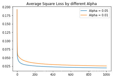
From this chart, we can find that the average square loss will not converge when Alpha = 0.5 or 0.1. Then we delete this two situations and show the situation of Alpha = 0.05 and 0.01 only. In this case, we can easily find out that when Alpha = 0.05 , the average square loss converge much quicker.

Implement backtracking line search

Here, $d$ is the gradient and $f(x)$ is the loss function. When $t\to 0$ we have :
$$f(t+t\Delta x)\approx f(x)+t\nabla f(x{)}^T$$
Assume $\gamma \in (0,1) , c \in (0,1) , \nu \in (0,1,2,…) $ we know that $ \gamma^\nu $ decreases as $\nu $ increases. So we increases the $\nu$ step by step in order find a $\nu $ that satisfy :
$$f(x_c+{\gamma }^{\nu }d)\ge f(x_c)+c{\gamma }^{\nu }{f}^{\prime }(x_c;d)$$
We have already know that $f^{\prime }(x_c;d)<0$ So, we can easily conclude that $f(x_c+{\gamma }^{\nu }d)\ge f(x_c)$

def backtracking_line_search(gamma, c, X, y, theta) :
    i = 1
    gradient = compute_square_loss_gradient(X, y, theta)
    function_deriv = compute_square_loss(X, y, theta-gradient)-compute_square_loss(X, y, theta)
    left = compute_square_loss(X, y, theta-gamma*gradient)
    right = compute_square_loss(X, y, theta)+c*gamma*function_deriv
    while left > right :
        i = i+1
        left = compute_square_loss(X, y, theta-pow(gamma, i)*gradient)
        right = compute_square_loss(X, y, theta)+c*pow(gamma, i)*function_deriv
    return pow(gamma, i)

def batch_grad_descent_with_backtracking(gamma, c, X, y, num_step) :
    num_instances, num_features = X.shape[0], X.shape[1]
    theta_hist = np.zeros((num_step+1, num_features)) #Initialize theta_hist
    loss_hist = np.zeros(num_step+1) #Initialize loss_hist
    theta = np.zeros(num_features) #Initialize theta
    step_size_hist = np.zeros(num_step) #Initialize step_size_hist
    
    theta_hist[0] = theta
    loss_hist[0] = compute_square_loss(X , y , theta)
        
    for i in range(num_step) :
        gradient = compute_square_loss_gradient(X , y , theta)
        alpha = backtracking_line_search(gamma, c, X, y, theta)
        step_size_hist[i] = alpha
        theta = theta - alpha*gradient
        theta_hist[i+1] = theta
        loss_hist[i+1] = compute_square_loss(X , y , theta)
    
    return theta_hist , loss_hist , step_size_hist

import time
start = time.clock()
batch_grad_descent(x_train, y_train, 0.06871948, 1000, False)
elapsed = time.clock()-start

start1 = time.clock()
batch_grad_descent_with_backtracking(0.8, 0.01, x_train, y_train, 1000)
elapsed1 = time.clock()-start1

print("Function without backtracking time used : ", elapsed)
print("Function with backtracking time used : ", elapsed1)
print("Extra time used : ", elapsed1 - elapsed)

Function without backtracking time used :  0.027063999999999977
Function with backtracking time used :  0.25299000000000005
Extra time used :  0.22592600000000007

From the result above, we find that it really takes time to find the best step size which will spend about ten times of time to get the result.

Part Five : Rigid Regression(i.e. Linear Regression with ${\ell }_2$ regularization)

When we have a large number of features compared to instances, regularization
can help control overfitting. Ridge regression is linear regression
with ${\ell }_2$ regularization. The regularization term is sometimes
called a penalty term. The objective function for ridge regression
is
$$J(\theta )=\frac{1}{m}\sum _{i=1}^m{\left(h_{\theta }(x_i)-y_i\right)}^2+\lambda {\theta }^T\theta ,$$
where $\lambda$ is the regularization parameter, which controls the
degree of regularization. Note that the bias parameter is being regularized
as well. We will address that below.

Firstly, we compute the gradient of $J(\theta )$ :

$$\begin{gathered} J(\theta +\eta h)=\frac{[(\theta +\eta h{)}^T{X}^{T}X(\theta +\eta h)-2y^{T}X(\theta +\eta h)+y^{T}y]}{m}+\lambda (\theta +\eta h{)}^T(\theta +\eta h) \\ \frac{J(\theta +\eta h)-J(\theta )}{\eta h}\approx 2{\theta }^2{X}^{T}X-2y^{T}X+2\lambda {\theta }^T \\ \nabla J(\theta )=2X^T(X\theta -y)+2\lambda \theta \end{gathered}$$

Function ：compute_regularized_square_loss(X, y, theta，lambda_reg)

Description : Given a set of X, y, theta, compute the average square loss for predicting y with $X\ast \theta$

Args:
    X - the feature vector, 2D numpy array of size (num_instances, num_features)
    y - the label vector, 1D numpy array of size (num_instances)
    theta - the parameter vector, 1D array of size (num_features)
    lambda_reg - the regularization coefficient

Returns:
    loss - the average square loss, scalar
loss = 0 (Initialize the average square loss)

def compute_regularized_square_loss(X, y, theta, lambda_reg) :
    regularized_square_loss = np.dot((np.dot(X , theta) - y).T , np.dot(X , theta) - y) / len(X) + lambda_reg*np.dot(theta.T, theta)
    return regularized_square_loss

Function : compute_regularized_square_loss_gradient(X, y, theta, lambda_reg)

Description : Compute the gradient of L2-regularized average square loss function given X, y and $\theta$

Args:
    X - the feature vector, 2D numpy array of size (num_instances, num_features)
    y - the label vector, 1D numpy array of size (num_instances)
    theta - the parameter vector, 1D numpy array of size (num_features)
    lambda_reg - the regularization coefficient

Returns:
    grad - gradient vector, 1D numpy array of size (num_features)

def compute_regularized_square_loss_gradient(X , y , theta , lambda_reg) :
    grad = 2*np.dot(X.T , np.dot(X , theta) - y) / len(X) + 2*lambda_reg*theta
    return grad

Function : regularized_grad_descent(X, y, alpha=0.05, lambda_reg=0.01, num_step=1000)

Description : Args:
X - the feature vector, 2D numpy array of size (num_instances, num_features)
y - the label vector, 1D numpy array of size (num_instances)
alpha - step size in gradient descent
lambda_reg - the regularization coefficient
num_step - number of steps to run

Returns:
    theta_hist - the history of parameter vector, 2D numpy array of size (num_step+1, num_features)
                 for instance, theta in step 0 should be theta_hist[0], theta in step (num_step+1) is theta_hist[-1]
    loss hist - the history of average square loss function without the regularization term, 1D numpy array.

def regularized_grad_descent(X , y , alpha , lambda_reg , num_step) :
    num_instances, num_features = X.shape[0] , X.shape[1]
    theta = np.zeros(num_features) #initialize theta
    theta_hist = np.zeros((num_step+1, num_features)) #Initialize theta_list
    loss_hist = np.zeros(num_step+1) #Initialize loss_hist
    
    theta_hist[0] = theta
    loss_hist[0] = compute_regularized_square_loss(X, y, theta, lambda_reg)
    
    for i in range(num_step) :
        gradient = compute_regularized_square_loss_gradient(X, y, theta, lambda_reg)
        theta = theta - alpha*gradient
        theta_hist[i+1] = theta
        loss_hist[i+1] = compute_regularized_square_loss(X, y, theta, lambda_reg)
        
    return theta_hist , loss_hist

Discussion I : How to deal with extra bias dimension? Why Regularization?

For regression problems, we may prefer to leave the bias term unregularized.
One approach is to change $J(\theta )$ so that the bias is separated
out from the other parameters and left unregularized. Another approach
that can achieve approximately the same thing is to use a very large
number $B$, rather than $1$, for the extra bias dimension.

For approach one, if we add a very large number multiply the ${\theta }_i$ we want to change, the average loss function will be like this :
$$J(\theta )=\frac{1}{m}\sum _{i=1}^m{\left(h_{\theta }(x_i)-y_i\right)}^2+1000{\theta }_i^2$$
if we want to minimize the average loss function, ${\theta }_i$ should be near zero and we can separate out the parameter from $\theta$ and let others unregularized

For approach two, if we want to use a very large number B, it will decrease the effective regularization.

Discussion II : How to find the best $\lambda$ ?

Set1 = np.array([10e-11, 10e-10, 10e-9, 10e-8, 10e-7, 10e-6, 10e-5, 10e-4, 10e-3, 10e-2, 0.1, 1])
Loss = np.zeros(len(Set1))
theta_List = np.zeros((len(Set1), x_train.shape[1]))
for i in range(len(Set1)) :
    a , b = regularized_grad_descent(x_train, y_train, 0.05, Set1[i], 1000)
    theta_List[i] = a[1000]
    Loss[i] = compute_regularized_square_loss(x_test, y_test, theta_List[i], Set1[i]) + Set1[i]*np.dot(theta_List[i].T, theta_List[i])
x = np.array([-11, -10, -9, -8, -7, -6, -5, -4, -3, -2, -1, 0])
y = Loss
plt.plot(x, y)
plt.xlabel('log(lambda)')
plt.ylabel('average square loss without regularization')
plt.title('Loss change as the increase in lambda')

Text(0.5,1,'Loss change as the increase in lambda')

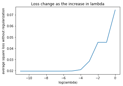
So in this case, we will choose $ \lambda = 10e-4$ as the lambda_reg parameter. Among those who gives us minimum average square loss on the test set, 10e-4 reaches the optimal point with least steps.

Part Six : Stochastic Gradient Descent

When the training data set is very large, evaluating the
gradient of the objective function can take a long time, since it
requires looking at each training example to take a single gradient
step. When the objective function takes the form of an average of
many values, such as
$$J(\theta )=\frac{1}{m}\sum _{i=1}^m{f}_i(\theta )$$
(as it does in the empirical risk), stochastic gradient descent (SGD)
can be very effective. In SGD, rather than taking $-\nabla J(\theta )$
as our step direction, we take $-\nabla f_i(\theta )$ for some $i$
chosen uniformly at random from { 1 , … , m } \{1,\ldots,m\} {1,…,m}. The approximation
is poor, but we will show it is unbiased.
In machine learning applications, each $f_i(\theta )$
would be the loss on the $i$th example (and of course we’d typically
write $n$ instead of $m$, for the number of training points). In
practical implementations for ML, the data points are randomly
shuffled, and then we sweep through the whole training set one by
one, and perform an update for each training example individually.
One pass through the data is called an epoch. Note that each
epoch of SGD touches as much data as a single step of batch gradient
descent. You can use the same ordering for each epoch, though optionally
you could investigate whether reshuffling after each epoch affects
the convergence speed.

Firstly we show that the objective function :
$$J(\theta )=\frac{1}{m}\sum _{i=1}^m{\left(h_{\theta }(x_i)-y_i\right)}^2+\lambda {\theta }^T\theta$$
can be written in the form $J(\theta )=\frac{1}{m}{\sum }_{i=1}^m{f}_i(\theta )$
by giving an expression for $f_i(\theta )$ that makes the two expressions
equivalent.

$$\begin{gathered} J(\theta )=\frac{1}{m}\sum _{i=1}^m[{\left(h_{\theta }(x_i)-y_i\right)}^2+\lambda m{\theta }^T\theta ] \\ J(\theta )=\frac{1}{m}\sum _{i=1}^m[(X_i\theta -y_i{)}^T(X_i\theta -y_i)+\lambda m{\theta }^T\theta ] \\ J(\theta )=\frac{1}{m}\sum _{i=1}^m{f}_i(\theta ) \end{gathered}$$

Secondly, we show that the stochastic gradient $\nabla f_i(\theta )$, for $i$
chosen uniformly at random from { 1 , … , m } \{1,\ldots,m\} {1,…,m}, is an unbiased
estimator of $\nabla J(\theta )$.

$$\begin{gathered} \nabla f_i(\theta )=2X_i(X_i\theta -y_i)+2\lambda m\theta \\ E[\nabla f_i(\theta )]=2E[X_i](E[X_i\theta -E[y_i])+2\lambda m\theta \\ E[\nabla f_i(\theta )]=\nabla J(\theta ) \end{gathered}$$

Now, we know how to compute the $\nabla f_{i}(\theta) $and use it to update $\theta$
$$\theta =\theta -\nabla f_i(\theta )$$
After that we can randomly select $X_i$ from the dataset, compute the gradient of the samples of each epoch and finally get the result

Function : stochastic_grad_descent(X, y, alpha=0.01, lambda_reg=0.01, num_epoch=1000)

Description : Implement stochastic gradient descent with regularization term

Args:
    X - the feature vector, 2D numpy array of size (num_instances, num_features)
    y - the label vector, 1D numpy array of size (num_instances)
    alpha - string or float, step size in gradient descent
            NOTE: In SGD, it's not a good idea to use a fixed step size. Usually it's set to 1/sqrt(t) or 1/t
            if alpha is a float, then the step size in every step is the float.
            if alpha == "1/sqrt(t)", alpha = 1/sqrt(t).
            if alpha == "1/t", alpha = 1/t.
    lambda_reg - the regularization coefficient
    num_epoch - number of epochs to go through the whole training set

Returns:
    theta_hist - the history of parameter vector, 3D numpy array of size (num_epoch, num_instances, num_features)
                 for instance, theta in epoch 0 should be theta_hist[0], theta in epoch (num_epoch) is theta_hist[-1]
    loss hist - the history of loss function vector, 2D numpy array of size (num_epoch, num_instances)

def stochastic_grad_descent(X, y, alpha, lambda_reg, num_epoch):
    num_instances, num_features = X.shape[0], X.shape[1]
    theta = np.ones(num_features) #Initialize theta
    
    theta_hist = np.zeros((num_epoch, num_instances, num_features)) #Initialize theta_hist
    loss_hist = np.zeros((num_epoch, num_instances)) #Initialize loss_hist
    
    y = y_train[:, np.newaxis]
    Sample = np.concatenate((X, y), axis = 1)
    
    for i in range(num_epoch) :
        np.random.shuffle(Sample)
        sample_x, sample_y = np.split(Sample, [-1], 1)
        sample_y = sample_y.squeeze()
        for j in range(num_instances) :
            sample_random = sample_x[j]
            theta = theta - alpha*compute_regularized_square_loss_gradient(sample_random, sample_y[j], theta, lambda_reg)
            theta_hist[i,j] = theta
            loss_hist[i,j] = compute_regularized_square_loss(sample_random, sample_y[j], theta, lambda_reg)
    
    return theta_hist, loss_hist

Will SGD converge if step size is fixed? Now Let’s try $\eta =0.05，0.005$

a, b = stochastic_grad_descent(x_train, y_train, 0.05, 0.01, 2)
c, d = stochastic_grad_descent(x_train, y_train, 0.005, 0.01, 2)
y1 = b.reshape(1, b.shape[0]*b.shape[1]).squeeze()
y2 = d.reshape(1, d.shape[0]*d.shape[1]).squeeze()
x = np.linspace(1, d.shape[0]*d.shape[1], d.shape[0]*d.shape[1])
plt.plot(x, y1, label = 'eta = 0.05' )
plt.plot(x, y2, label = 'eta = 0.005')
plt.xlabel('time')
plt.ylabel('loss')
plt.legend()
plt.show()

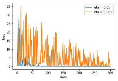
So we learn from the graph above that SGD may not converge with the fixed step size. Next we try step sizes that decrease with the step number according to the following schedules: ${\eta }_t=\frac{C}{t}$ and ${\eta }_t=\frac{C}{\sqrt{t}}$, $C\le 1$.

def SGD_first(X, y, alpha, lambda_reg, num_epoch) :
    num_instances, num_features = X.shape[0], X.shape[1]
    theta = np.ones(num_features) #Initialize theta
    
    theta_hist = np.zeros((num_epoch, num_instances, num_features)) #Initialize theta_hist
    loss_hist = np.zeros((num_epoch, num_instances)) #Initialize loss_hist
    
    y = y_train[:, np.newaxis]
    Sample = np.concatenate((X, y), axis = 1)
    
    for i in range(num_epoch) :
        np.random.shuffle(Sample)
        sample_x, sample_y = np.split(Sample, [-1], 1)
        sample_y = sample_y.squeeze()
        for j in range(num_instances) :
            sample_random = sample_x[j]
            theta = theta - alpha/pow(i+1, 0.5)*compute_regularized_square_loss_gradient(sample_random, sample_y[j], theta, lambda_reg)
            theta_hist[i,j] = theta
            loss_hist[i,j] = compute_regularized_square_loss(sample_random, sample_y[j], theta, lambda_reg)
    
    return theta_hist, loss_hist

def SGD_second(X, y, alpha, lambda_reg, num_epoch) :
    num_instances, num_features = X.shape[0], X.shape[1]
    theta = np.ones(num_features) #Initialize theta
    
    theta_hist = np.zeros((num_epoch, num_instances, num_features)) #Initialize theta_hist
    loss_hist = np.zeros((num_epoch, num_instances)) #Initialize loss_hist
    
    y = y_train[:, np.newaxis]
    Sample = np.concatenate((X, y), axis = 1)
    
    for i in range(num_epoch) :
        np.random.shuffle(Sample)
        sample_x, sample_y = np.split(Sample, [-1], 1)
        sample_y = sample_y.squeeze()
        for j in range(num_instances) :
            sample_random = sample_x[j]
            theta = theta - alpha/(i+1)*compute_regularized_square_loss_gradient(sample_random, sample_y[j], theta, lambda_reg)
            theta_hist[i,j] = theta
            loss_hist[i,j] = compute_regularized_square_loss(sample_random, sample_y[j], theta, lambda_reg)
    
    return theta_hist, loss_hist

a, b = SGD_first(x_train, y_train, 0.1, 0.01, 2)
c, d = stochastic_grad_descent(x_train, y_train, 0.1, 0.01, 2)
y1 = b.reshape(1, b.shape[0]*b.shape[1]).squeeze()
y2 = d.reshape(1, d.shape[0]*d.shape[1]).squeeze()
x = np.linspace(1, d.shape[0]*d.shape[1], d.shape[0]*d.shape[1])
plt.plot(x, y1, label = 'C/t' )
plt.plot(x, y2, label = 'C/sqrt(t)')
plt.xlabel('time')
plt.ylabel('loss')
plt.legend()
plt.show()

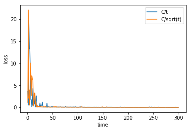
From the graph above, we can find that after adjusting the alpha, SGD converges much more quickly.

Part Seven : Risk Minimization

Square Loss

Let $y$ be a random variable with a known distribution, and consider the square loss function $\ell (a,y)=(a-y{)}^2$. We want to find the action $a^{\ast }$ that has minimal risk. That is, we want to find $a^{\ast }=argmi{n}_{a}E{\left(a-y\right)}^2$, where the expectation is with respect to $y$. Now, we show that $a^{\ast }=y$, and the Bayes risk (i.e. the risk of $a^{\ast }$) is $Var(y)$.

$$minE(a-y{)}^2=minE(|a-y|)=minE(|a-E(y)|)\Rightarrow a^{\ast }=E(y)$$

$$E[E(y)-y{]}^2=E[y^2]-2E[y{]}^2+E[y{]}^2=E[y^2]-E[y{]}^2=Var(y)$$

Now let’s introduce an input. Recall that the expected loss or '‘risk’'of a decision function $f:X\to A$ is
$$R(f)=E\ell (f(x),y)$$
where $(x,y)\sim P_{X\times Y}$, and the Bayes decision function $f^{\ast }:X\to A$ is a function that achieves the minimal
risk among all possible functions:
$$R(f^{\ast })=\underset{f}{\inf }R(f)$$
Here we consider the regression setting, in which $A=Y=R$. We will show for the square loss $\ell (a,y)={\left(a-y\right)}^2$, the Bayes decision function is $f^{\ast }(x)=E\left[y\mid x\right]$, where the expectation is over $y$. As before, we assume we know the data-generating distribution $P_{X\times Y}$.

We’ll approach this problem by finding the optimal action for any given $x$. If somebody tells us $x$, we know that the corresponding $y$ is coming from the conditional distribution $y\mid x$. For a particular $x$, what value should we predict (i.e. what action $a$ should we produce) that has minimal expected loss? In mathematical notation, we’re looking for :
$$f^{\ast }(x)=argmi{n}_{a}E\left[{\left(a-y\right)}^2\mid x\right]$$
where the expectation is with respect to $y$.

From the previous part, we know $a^* $ is the expectation of $y$ , here, the same, we get :

$$a^{\ast }=E[Y|X]$$

In the previous problem we produced a decision function $f^{\ast }(x)$ that minimized the risk for each $x$. In other words, for any other decision function $f(x)$, $f^{\ast }(x)$ is going to be at least as good as $f(x)$, for every single $x$. In math, we mean
$$E\left[{\left(f^{\ast }(x)-y\right)}^2\mid x\right]\le E\left[{\left(f(x)-y\right)}^2\mid x\right],$$
for all $x$. To show that $f^{\ast }(x)$ is the Bayes decision function, we need to show that
$$E\left[{\left(f^{\ast }(x)-y\right)}^2\right]\le E\left[{\left(f(x)-y\right)}^2\right]$$
for any $f$.

Implement Law of iterated expectations :

$$E\left[E\left[{\left(f^{\ast }(x)-y\right)}^2\mid x\right]\right]\le E\left[E\left[{\left(f(x)-y\right)}^2\mid x\right]\right],$$

$$E\left[{\left(f^{\ast }(x)-y\right)}^2\right]\le E\left[{\left(f(x)-y\right)}^2\right]$$