从0开始入门数据挖掘(三)-模型和调参

最新推荐文章于 2025-01-02 14:49:38 发布

yuting_

最新推荐文章于 2025-01-02 14:49:38 发布

阅读量348

点赞数

分类专栏：机器学习

本文链接：https://blog.youkuaiyun.com/weixin_38120348/article/details/105230505

版权

机器学习专栏收录该内容

13 篇文章

订阅专栏

本文将以天池的一道赛题入手，详细介绍数据挖掘的步骤，实际操作性强。

适合人群：想入门数据挖掘，入门数据挖掘类比赛，熟悉python，pandas，Numpy等库运用性选手

本文是从0开始入门数据挖掘系列文章的第三篇，第一篇介绍的是EDA部分，也就是数据探索性分析，第二篇介绍了特征工程，这一篇文章将给大家介绍模型和调参。

内容介绍：

简单模型
模型性能验证
嵌入式特征选择（继上篇的特征选择-过滤式(Filter)、包裹式(Wrapper)的第三种特征选择方法）
模型对比
模型调参
- 贪心调参方法；
- 网格调参方法；
- 贝叶斯调参方法；

1.简单模型

由于此次的竞赛题为回归问题，所以拿解决回归问题最经典的算法——线性回归来介绍，帮助理解机器学习模型的建模与调参流程。

from sklearn.linear_model import LinearRegression

model = LinearRegression(normalize=True)
model = model.fit(train_X, train_y)

# 查看训练的线性回归模型的截距（intercept）与权重(coef)¶
'intercept'+str(model.intercept_)
# key= lambda x : x[1]把Key换成权重 然后按照权重排序
sorted(dict(zip(continuous_feature_names, model.coef_)).items(), key= lambda x : x[1], reverse = True) 

from matplotlib import pyplot as plt
subsample_index = np.random.randint(low=0, high=len(train_y),size=50) # 大小为50

plt.scatter(train_X['v_9'][subsample_index],train_y[subsample_index], color='black')
plt.scatter(train_X['v_9'][subsample_index],model.predict(train_X.loc[subsample_index]), color='blue')
plt.xlabel('v_9')
plt.ylabel('price')
plt.legend(['True Price','Predicted Price'],loc='upper right')  # 加上右上角的标签
print('The predicted price is obvious different from true price')
plt.show()

import seaborn as sns
%matplotlib inline
print('It is clear to see the price shows a typical exponential distribution')
plt.figure(figsize=(15,5))  # 设置画布大小
plt.subplot(1,2,1) # 子图
sns.distplot(train_y)
plt.subplot(1,2,2) # 子图
sns.distplot(train_y[train_y < np.quantile(train_y, 0.9)])

在这里插入图片描述
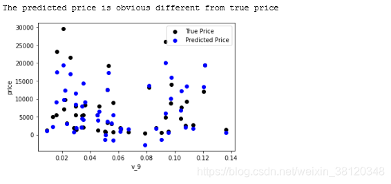
上图可发现，训练出来的模型对验证数据拟合效果不好。

我们看看预测price值的分布情况和去掉长尾后的分布情况

import seaborn as sns
%matplotlib inline
print('It is clear to see the price shows a typical exponential distribution')
plt.figure(figsize=(15,5))  # 设置画布大小
plt.subplot(1,2,1) # 子图
sns.distplot(train_y)
plt.subplot(1,2,2) # 子图
sns.distplot(train_y[train_y < np.quantile(train_y, 0.9)])

在这里插入图片描述
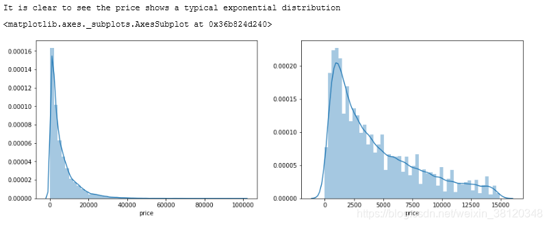
通过作图我们发现数据的标签（price）呈现长尾分布，不利于我们的建模预测。原因是很多模型都假设数据误差项符合正态分布，而长尾分布的数据违背了这一假设
参考博客：https://blog.youkuaiyun.com/Noob_daniel/article/details/76087829

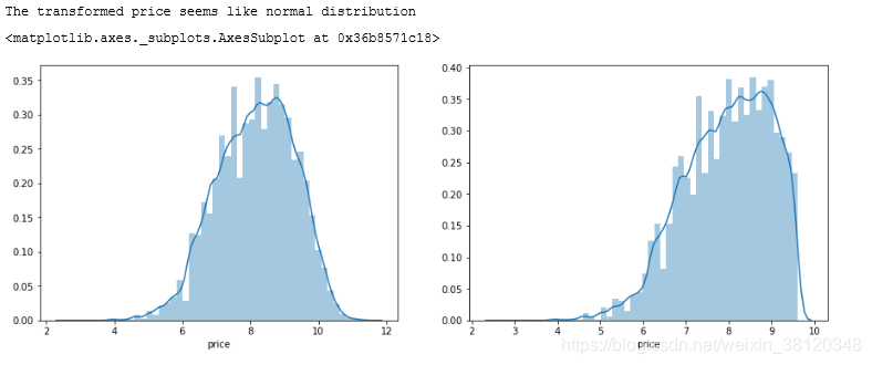
在这里我们对标签进行了 log(x+1) 变换，使标签贴近于正态分布

train_y_ln = np.log(train_y+1)

import seaborn as sns
print('The transformed price seems like normal distribution')
plt.figure(figsize=(15,5))
plt.subplot(1,2,1)
sns.distplot(train_y_ln)
plt.subplot(1,2,2)
sns.distplot(train_y_ln[train_y_ln < np.quantile(train_y_ln, 0.9)])

model = model.fit(train_X, train_y_ln)

print('intercept:'+ str(model.intercept_))
sorted(dict(zip(continuous_feature_names, model.coef_)).items(), key=lambda x:x[1], reverse=True)

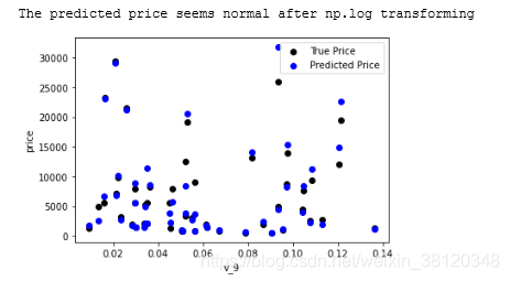
plt.scatter(train_X['v_9'][subsample_index], train_y[subsample_index], color='black')
plt.scatter(train_X['v_9'][subsample_index], np.exp(model.predict(train_X.loc[subsample_index])), color='blue')
plt.xlabel('v_9')
plt.ylabel('price')
plt.legend(['True Price','Predicted Price'],loc='upper right')
print('The predicted price seems normal after np.log transforming')
plt.show()

在这里插入图片描述

2.模型性能验证

模型训练-五折交叉验证

from sklearn.model_selection import cross_val_score
from sklearn.metrics import mean_absolute_error, make_scorer

def log_transfer(func):
    def wrapper(y, yhat):
        result = func(np.log(y),np.nan_to_num(np.log(yhat)))
        return result
    return wrapper

#  cross_val_score的返回值是一个数组，数组中的元素是每次交叉检验模型的得分。
# scoring:需要string, callable or None，表示通过哪个机制来打分
# cv: 需要int，cross_validation generator or an iterable，默认为3重交叉检验
scores = cross_val_score(model, X=train_X, y=train_y, verbose=1, cv = 5, scoring=make_scorer(log_transfer(mean_absolute_error)))

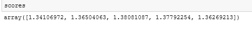
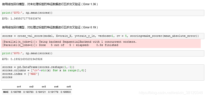
#使用线性回归模型，对未处理标签的特征数据进行五折交叉验证（Error 1.36）
print('AVG:', np.mean(scores))
#使用线性回归模型，对处理过标签的特征数据进行五折交叉验证（Error 0.19）
scores = cross_val_score(model, X=train_X, y=train_y_ln, verbose=1, cv = 5, scoring=make_scorer(mean_absolute_error))

print('AVG:', np.mean(scores))
# AVG: 0.19321630231943926

scores = pd.DataFrame(scores.reshape(1,-1))
scores.columns = ['cv'+str(x) for x in range(1,6)]
scores.index = ['MAE']
scores

在这里插入图片描述

注意：在使用五折交叉验证对时间相关的数据集进行预测时：

越靠近预测时间的训练数据往往会得到更好的效果，所以拿今年上半年的销售数据来预测今年下半年的销售情况会比拿去年的数据要好（不考虑周期性）。

因此我们还可以采用时间顺序对数据集进行分隔，在本例中，我们选用靠前时间的4/5样本当作训练集，靠后时间的1/5当作验证集

import datetime
sample_feature = sample_feature.reset_index(drop=True)
split_point = len(sample_feature)//5*4

train = sample_feature.loc[:split_point].dropna()
val = sample_feature.loc[split_point:].dropna()

train_X = train[continuous_feature_names]
train_y_ln = np.log(train['price'] + 1)
val_X = val[continuous_feature_names]
val_y_ln = np.log(val['price'] + 1)

model = model.fit(train_X, train_y_ln)
mean_absolute_error(val_y_ln, model.predict(val_X))

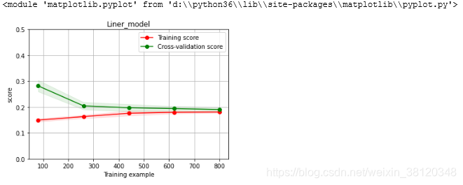
绘制学习率曲线与验证曲线

from sklearn.model_selection import learning_curve, validation_curve

def plot_learning_curve(estimator, title, X, y, ylim=None, cv=None,n_jobs=1, train_size=np.linspace(.1, 1.0, 5 )):  
    plt.figure()  
    plt.title(title)  
    if ylim is not None:  
        plt.ylim(*ylim)  
    plt.xlabel('Training example')  
    plt.ylabel('score')  
    train_sizes, train_scores, test_scores = learning_curve(estimator, X, y, cv=cv, n_jobs=n_jobs, train_sizes=train_size, scoring = make_scorer(mean_absolute_error))  
    train_scores_mean = np.mean(train_scores, axis=1)  
    train_scores_std = np.std(train_scores, axis=1)  
    test_scores_mean = np.mean(test_scores, axis=1)  
    test_scores_std = np.std(test_scores, axis=1)  
    plt.grid()#区域  
    plt.fill_between(train_sizes, train_scores_mean - train_scores_std,  
                     train_scores_mean + train_scores_std, alpha=0.1,  
                     color="r")  
    plt.fill_between(train_sizes, test_scores_mean - test_scores_std,  
                     test_scores_mean + test_scores_std, alpha=0.1,  
                     color="g")  
    plt.plot(train_sizes, train_scores_mean, 'o-', color='r',  
             label="Training score")  
    plt.plot(train_sizes, test_scores_mean,'o-',color="g",  
             label="Cross-validation score")  
    plt.legend(loc="best")  
    return plt  

plot_learning_curve(LinearRegression(), 'Liner_model', train_X[:1000], train_y_ln[:1000], ylim=(0.0, 0.5), cv=5, n_jobs=1)

在这里插入图片描述

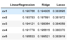
3.嵌入式特征选择-嵌入式特征选择

嵌入式特征选择在学习器训练过程中自动地进行特征选择。嵌入式选择最常用的是L1正则化与L2正则化。在对线性回归模型加入两种正则化方法后，他们分别变成了岭回归与Lasso回归。

from sklearn.linear_model import LinearRegression
from sklearn.linear_model import Ridge
from sklearn.linear_model import Lasso

models = [LinearRegression(),
          Ridge(),
          Lasso()]

result = dict()
for model in models:
    model_name = str(model).split('(')[0]
    scores = cross_val_score(model, X=train_X, y=train_y_ln, verbose=0, cv = 5, scoring=make_scorer(mean_absolute_error))
    result[model_name] = scores
    print(model_name + ' is finished')

#三种方法的效果对比
result = pd.DataFrame(result)
result.index = ['cv' + str(x) for x in range(1, 6)]
result

在这里插入图片描述

model = LinearRegression().fit(train_X, train_y_ln)
print('intercept:'+ str(model.intercept_))
sns.barplot(abs(model.coef_), continuous_feature_names)

在这里插入图片描述

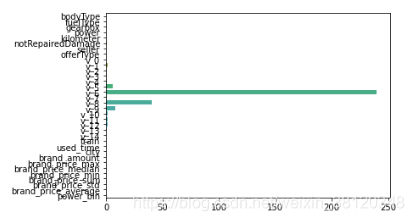
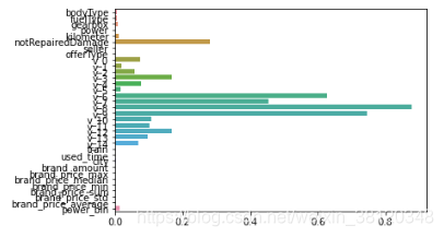
L2正则化在拟合过程中通常都倾向于让权值尽可能小，最后构造一个所有参数都比较小的模型。因为一般认为参数值小的模型比较简单，能适应不同的数据集，也在一定程度上避免了过拟合现象

model = Ridge().fit(train_X, train_y_ln)
print('intercept:'+ str(model.intercept_))
sns.barplot(abs(model.coef_), continuous_feature_names)

在这里插入图片描述

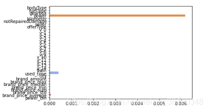
L1正则化适用于稀疏权值矩阵，进而可以用于特征选择。如下图，我们发现power与userd_time特征非常重要

model = Lasso().fit(train_X, train_y_ln)
print('intercept:'+ str(model.intercept_))
sns.barplot(abs(model.coef_), continuous_feature_names)

在这里插入图片描述

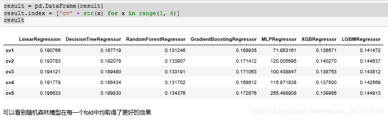
4. 模型对比

以下为线性回归、决策树、随机森林、xgboost、lgbm等模型训练情况对比：

from sklearn.linear_model import LinearRegression
from sklearn.svm import SVC
from sklearn.tree import DecisionTreeRegressor
from sklearn.ensemble import RandomForestRegressor
from sklearn.ensemble import GradientBoostingRegressor
from sklearn.neural_network import MLPRegressor
from xgboost.sklearn import XGBRegressor
from lightgbm.sklearn import LGBMRegressor

models = [LinearRegression(),
          DecisionTreeRegressor(),
          RandomForestRegressor(),
          GradientBoostingRegressor(),
          MLPRegressor(solver='lbfgs', max_iter=100), 
          XGBRegressor(n_estimators = 100, objective='reg:squarederror'), 
          LGBMRegressor(n_estimators = 100)]

result = dict()
for model in models:
    model_name = str(model).split('(')[0]
    scores = cross_val_score(model,X = train_X, y=train_y_ln, verbose=0,cv=5,scoring=make_scorer(mean_absolute_error))
    result[model_name] = scores
    print(model_name + ' is finished')

result = pd.DataFrame(result)
result.index = ['cv' + str(x) for x in range(1, 6)]
result

在这里插入图片描述

5. 模型调参

贪心调参

## LGB的参数集合：

objective = ['regression', 'regression_l1', 'mape', 'huber', 'fair']
num_leaves = [3,5,10,15,20,40, 55]
max_depth = [3,5,10,15,20,40, 55]
bagging_fraction = []
feature_fraction = []
drop_rate = []


best_obj = dict()
for obj in objective:
    model = LGBMRegressor(objective=obj)
    score = np.mean(cross_val_score(model, X=train_X, y=train_y_ln, verbose=0, cv = 5, scoring=make_scorer(mean_absolute_error)))
    best_obj[obj] = score
    
best_leaves = dict()
for leaves in num_leaves:
    model = LGBMRegressor(objective=min(best_obj.items(), key=lambda x:x[1])[0], num_leaves=leaves)
    score = np.mean(cross_val_score(model, X=train_X, y=train_y_ln, verbose=0, cv = 5, scoring=make_scorer(mean_absolute_error)))
    best_leaves[leaves] = score
    
best_depth = dict()
for depth in max_depth:
    model = LGBMRegressor(objective=min(best_obj.items(), key=lambda x:x[1])[0],
                          num_leaves=min(best_leaves.items(), key=lambda x:x[1])[0],
                          max_depth=depth)
    score = np.mean(cross_val_score(model, X=train_X, y=train_y_ln, verbose=0, cv = 5, scoring=make_scorer(mean_absolute_error)))
    best_depth[depth] = score

Grid Search 调参

from sklearn.model_selection import GridSearchCV

parameters = {'objective': objective , 'num_leaves': num_leaves, 'max_depth': max_depth}
model = LGBMRegressor()
#网格搜索
clf = GridSearchCV(model, parameters, cv=5)
clf = clf.fit(train_X, train_y)

clf.best_params_
# {'max_depth': 15, 'num_leaves': 55, 'objective': 'regression'}

#将得到的最好参数传入模型
model = LGBMRegressor(objective='regression',
                          num_leaves=55,
                          max_depth=15)
                        
np.mean(cross_val_score(model, X=train_X, y=train_y_ln, verbose=0, cv = 5, scoring=make_scorer(mean_absolute_error)))

贝叶斯调参

from bayes_opt import BayesianOptimization

def rf_cv(num_leaves, max_depth, subsample, min_child_samples):
    val = cross_val_score(
        LGBMRegressor(objective = 'regression_l1',
            num_leaves=int(num_leaves),
            max_depth=int(max_depth),
            subsample = subsample,
            min_child_samples = int(min_child_samples)
        ),
        X=train_X, y=train_y_ln, verbose=0, cv = 5, scoring=make_scorer(mean_absolute_error)
    ).mean()
    return 1 - val

rf_bo = BayesianOptimization(
    rf_cv,
    {
    'num_leaves': (2, 100),
    'max_depth': (2, 100),
    'subsample': (0.1, 1),
    'min_child_samples' : (2, 100)
    }
)

rf_bo.maximize()

1 - rf_bo.max['target']
# 0.1296693644053145