机器学习多变量线性回归代码_机器学习单变量线性回归

机器学习多变量线性回归代码

Linear Regression (LR) is one of the main algorithms in Supervised Machine Learning. It solves many regression problems and it is easy to implement. This paper is about Univariate Linear Regression(ULR) which is the simplest version of LR.

线性回归(LR)是监督机器学习中的主要算法之一。 它解决了许多回归问题，并且易于实现。 本文是关于单变量线性回归(ULR)，它是LR的最简单版本。

The paper contains following topics:

本文包含以下主题：

• The basics of datasets in Machine Learning;
  机器学习中数据集的基础；
• What is Univariate Linear Regression?
  什么是单变量线性回归？
• How to represent the algorithm(hypothesis), Graphs of functions;
  如何表示算法(假设)，函数图；
• Cost function (Loss function);
  成本函数(损失函数)；
• Gradient Descent.
  梯度下降。

机器学习中的数据集基础 (The basics of datasets in Machine Learning)

In ML problems, beforehand some data is provided to build the model upon. The datasets contain of rows and columns. Each row represents an example, while every column corresponds to a feature.

在ML问题中，事先会提供一些数据以建立模型。 数据集包含行和列。 每行代表一个示例，而每列代表一个特征。

Then the data is divided into two parts — training and test sets. With percent, training set contains approximately 75%, while test set has 25% of total data. Training set is used to build the model. After model return success percent over about 90–95% on training set, it is tested with test set. Result with test set is considered more valid, because data in test set is absolutely new to the model.

然后将数据分为两个部分-训练集和测试集。 如果使用百分比，则训练集约占75％，而测试集占总数据的25％。 训练集用于构建模型。 在训练集上模型返回成功率超过大约90–95％之后，将使用测试集对其进行测试。 带有测试集的结果被认为更有效，因为测试集中的数据对于模型而言绝对是新的。

什么是单变量线性回归？ (What is Univariate Linear Regression?)

In Machine Learning problems, the complexity of algorithm depends on the provided data. When LR is used to build the ML model, if the number of features in training set is one, it is called Univariate LR, if the number is higher than one, it is called Multivariate LR. To learn Linear Regression, it is a good idea to start with Univariate Linear Regression, as it simpler and better to create first intuition about the algorithm.

在机器学习问题中，算法的复杂性取决于所提供的数据。 当使用LR构建ML模型时，如果训练集中的特征数为1，则称为Univariate LR；如果数量大于1，则称为Multivariate LR。 要学习线性回归，从单变量线性回归开始是一个好主意，因为创建有关该算法的第一个直觉会更简单，更好。

假设图 (Hypothesis, graphs)

To get intuitions about the algorithm I will try to explain it with an example. The example is a set of data on Employee Satisfaction and Salary level.

为了获得有关算法的直觉，我将尝试通过一个示例进行解释。 该示例是一组有关员工满意度和薪资水平的数据。

Figure 1. Raw dataset

图1.原始数据集

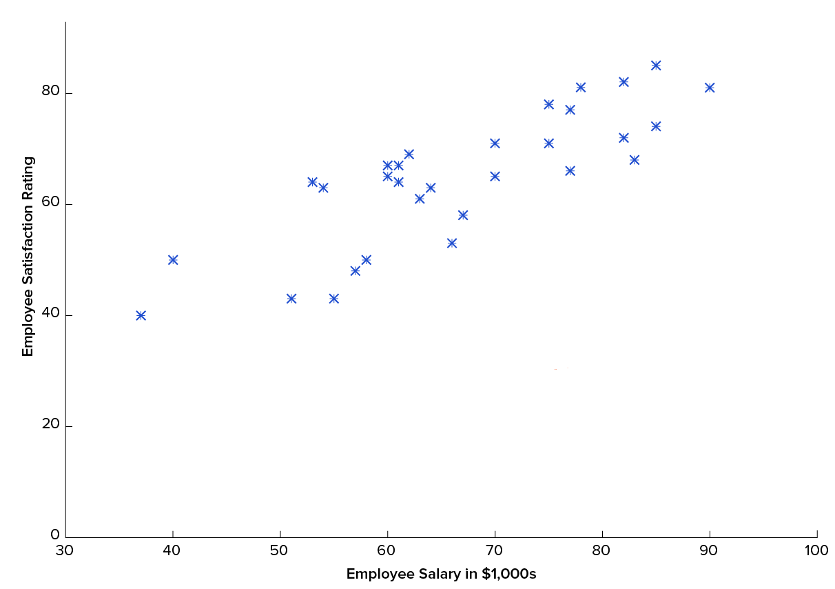
As it is seen from the picture, there is linear dependence between two variables. Here Employee Salary is a “X value”, and Employee Satisfaction Rating is a “Y value”. In this particular case there is only one variable, so Univariate Linear Regression can be used in order to solve this problem.

从图片中可以看出，两个变量之间存在线性关系。 在这里，员工薪水是“ X值”，员工满意度等级是“ Y值”。 在此特定情况下，只有一个变量，因此可以使用单变量线性回归来解决此问题。

In the following picture you will see three different lines.

在下图中，您将看到三行不同的内容。

Figure 2. 3 lines on the dataset

图2.数据集上的3行

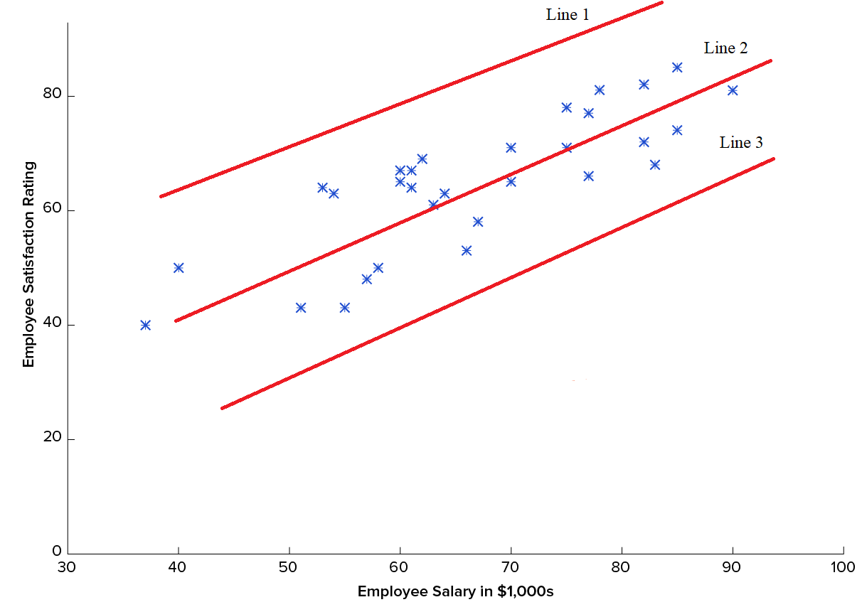
This is already implemented ULR example, but we have three solutions and we need to choose only one of them. Visually we can see that Line 2 is the best one among them, because it fits the data better than both Line 1 and Line 3. This is rather easier decision to make and most of the problems will be harder than that. The following paragraphs are about how to make these decisions precisely with the help of mathematical solutions and equations.

这已经实现了ULR示例，但是我们有三种解决方案，我们只需要选择其中一种即可。 从视觉上我们可以看到，第2行是其中最好的一条，因为它比第1行和第3行都更适合数据。这是比较容易做出的决定，而且大多数问题都比这困难。 以下各段是关于如何借助数学解和方程式精确地做出这些决定的。

Now let’s see how to represent the solution of Linear Regression Models (lines) mathematically:

现在，让我们看看如何用数学方法表示线性回归模型(线)的解：

Here,

这里，

• hθ(x) — the answer of the hypothesis
  hθ(x)-假设的答案

• θ0 and θ1 — parameters we have to calculate to fit the line to the data

  θ0和θ1 —我们必须计算的参数才能使线适合数据

• x — the point from the dataset

  x-数据集中的点

This is exactly same as the equation of line — y = mx + b. As the solution of Univariate Linear Regression is a line, equation of line is used to represent the hypothesis(solution).

这与线y = mx + b的方程式完全相同。 由于单变量线性回归的解是一条线，因此使用线方程表示假设(解)。

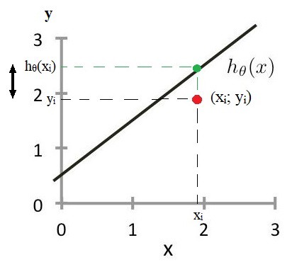
Let’s look at an example. For instance, there is a point in the provided training set — (x = 1.9; y = 1.9) and the hypothesis of h(x) = -1.3 + 2x. When this hypothesis is applied to the point, we get the answer of approximately 2.5.

让我们来看一个例子。 例如，所提供的训练集中有一个要点-(x = 1.9; y = 1.9)， h(x)的假设是-1.3 + 2x 。 将这一假设应用于该点时，我们得到的答案约为2.5。

After the answer is got, it should be compared with y value (1.9 in the example) to check how well the equation works. In this particular example there is difference of 0.6 between real value — y, and the hypothesis. So for this particular case 0.6 is a big difference and it means we need to improve the hypothesis in order to fit it to the dataset better.

得到答案后，应将其与y值(本例中为1.9)进行比较，以检查方程的工作效果。 在此特定示例中，实际值y与假设之间存在0.6的差异。 因此，对于这种特殊情况，0.6是一个很大的差异，这意味着我们需要改进假设以使其更好地适合数据集。

But here comes the question — how can the value of h(x) be manipulated to make it as possible as close to y? In order to answer the question, let’s analyze the equation. There are three parameters — θ0, θ1, and x. X is from the dataset, so it cannot be changed (in example the pair is (1.9; 1.9), and if you get h(x) = 2.5, you cannot change the point to (1.9; 2.5)). So we left with only two parameters (θ0 and θ1) to optimize the equation. In optimization two functions — Cost function and Gradient descent, play important roles, Cost function to find how well the hypothesis fit the data, Gradient descent to improve the solution.

但是，这里出现了一个问题–如何操纵h(x)的值以使其尽可能接近y？ 为了回答这个问题，让我们分析方程式。 有三个参数- θ0，θ1，并且x。 X来自数据集，因此无法更改(例如，对为(1.9; 1.9)，如果得到h(x)= 2.5，则无法将点更改为(1.9; 2.5))。 所以我们只剩下两个参数( θ0和 θ1)，以优化方程。 在优化中，两个函数-Cost函数和Gradient下降起着重要作用，Cost函数用于查找假设与数据的拟合程度，Gradient下降以改善求解。

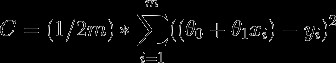
成本函数(损失函数) (Cost function (Loss function))

In the examples above, we did some comparisons in order to determine whether the line is fit to the data or not. In the first one, it was just a choice between three lines, in the second, a simple subtraction. But how will we evaluate models for complicated datasets? It is when Cost function comes to aid. In a simple definition, Cost function evaluates how well the model (line in case of LR) fits to the training set. There are various versions of Cost function, but we will use the one below for ULR:

在上面的示例中，我们进行了一些比较，以确定该行是否适合数据。 在第一行中，它只是三行之间的选择，在第二行中，是简单的减法。 但是，我们将如何评估复杂数据集的模型？ 这是成本函数提供帮助的时候。 在一个简单的定义中，成本函数评估模型(对于LR而言，线)与训练集的拟合程度。 Cost函数有多种版本，但是我们将在ULR中使用以下版本：

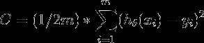
Here,

这里，

• m — number of examples in training set;
  m-训练集中的示例数；

• h — answer of hypothesis;

  h-假设的答案；

• y — y values of points in the dataset.

  y —数据集中点的y值。

The optimization level of the model is related with the value of Cost function. The smaller the value is, the better the model is. Why? The answer is simple — Cost is equal to the sum of the squared differences between value of the hypothesis and y. If all the points were on the line, there will not be any difference and answer would be zero. To put it another way, if the points were far away from the line, the answer would be very large number. To sum up, the aim is to make it as small as possible.

模型的优化水平与成本函数的值有关。 值越小，模型越好。 为什么？ 答案很简单-成本等于假设值与y之间的平方差之和。 如果所有点都在线上，则不会有任何差异，答案将为零。 换句话说，如果点离线很远，答案将是非常大的。 综上所述，目的是使其尽可能小。

So, from this point, we will try to minimize the value of the Cost function.

因此，从这一点出发，我们将尝试最小化Cost函数的值。

梯度下降 (Gradient Descent)

In order to get proper intuition about Gradient Descent algorithm let’s first look at some graphs.

为了获得关于梯度下降算法的正确直觉，让我们首先看一些图。

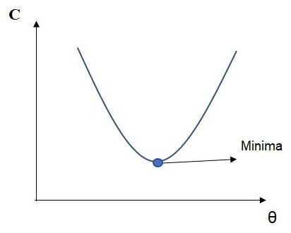
This is dependence graph of Cost function from theta. As mentioned above, the optimal solution is when the value of Cost function is minimum. In Univariate Linear Regression the graph of Cost function is always parabola and the solution is the minima.

这是Theta的Cost函数的依赖图。 如上所述，最佳解决方案是Cost函数的值最小时。 在单变量线性回归中，Cost函数的图形始终为抛物线，且解为最小值。

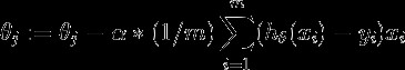
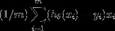
Gradient Descent is the algorithm such that it finds the minima:

梯度下降是找到最小值的算法：

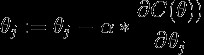
Here,

这里，

• α — learning rate;
  α-学习率；

The equation may seem a little bit confusing, so let’s go over step by step.

该方程式似乎有些令人困惑，所以让我们逐步进行研究。

1. What is this symbol — ‘:=’?
   这个符号是什么-'：='？

• Firstly, it is not same as ‘=’. ‘:=’ means “to update the left side value”, here it is not possible to use ‘=’ mathematically, because a number cannot be equal to subtraction of itself and something else (zero is an exception in this case).

  首先，它与'='不同。 '：='表示“更新左侧值” ，此处无法在数学上使用'='，因为数字不能等于其自身和其他东西的减法(在这种情况下，零是一个例外)。

2. What is ‘j’?

2.什么是“ j” ？

• ‘j’ is related to the number of features in the dataset. In Univariate Linear Regression there is only one feature and j is equal to 2. ‘j’ = number of features + 1.

  “ j”与数据集中的要素数量有关。 在单变量线性回归中，只有一个特征，并且j等于2 。 'j'=特征数量+ 1。

3. What is ‘alpha’?

3.什么是“ alpha”？

• ‘alpha’ is learning rate. Its value is usually between 0.001 and 0.1 and it is a positive number. If it is high the algorithm may ‘jump’ over the minima and diverge from solution. If it is low the convergence will be slow. In most cases several instances of ‘alpha’ is tired and the best one is picked.
  “ alpha”是学习率。 它的值通常在0.001和0.1之间，并且是一个正数。 如果该值很高，则该算法可能会“跳过”最小值并偏离解。 如果该值较低，则收敛速度将很慢。 在大多数情况下，“ alpha”的几种情况很累，最好的一种被选中。

4. The term of partial derivative.

4.偏导数项。

• Cost function mentioned above:
  上面提到的成本函数：

• Cost function with definition of h(x) substituted:

  定义了h(x)的成本函数：

• Derivative of Cost function:
  成本函数的导数：

5. Why is derivative used and sing before alpha is negative?

5.为什么在alpha为负数之前使用导数并唱歌？

• The answer of the derivative is the slope. The example graphs below show why derivate is so useful to find the minima.
  导数的答案是斜率。 下面的示例图显示了为什么求导如此有用以找到最小值。

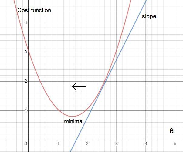
In the first graph above, the slope — derivative is positive. As is seen, the interception point of line and parabola should move towards left in order to reach optima. For that, the X value(theta) should decrease. Now let’s remember the equation of the Gradient descent — alpha is positive, derivative is positive (for this example) and the sign in front is negative. Overall the value is negative and theta will be decreased.

在上面的第一张图中，斜率-导数为正。 如图所示，线和抛物线的截取点应向左移动以达到最佳状态。 为此，X值θ应减小。 现在，让我们记住梯度下降的方程式-alpha为正，导数为正(在此示例中)，前面的符号为负。 总体而言，该值为负，θ将减小。

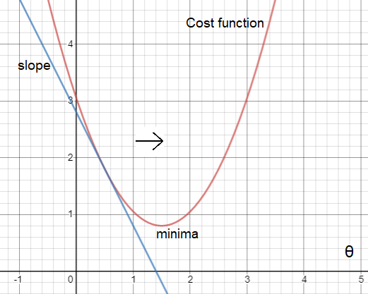
In the second example, the slope — derivative is negative. As is seen, the interception point of line and parabola should move towards right in order to reach optima. For that, the X value(theta) should increase. Now let’s remember the equation of the Gradient descent — alpha is positive, derivative is negative (for this example) and the sign in front is negative. Overall the value is positive and theta will be increased.

在第二个示例中，斜率-导数为负。 如图所示，直线和抛物线的截取点应向右移动以达到最佳状态。 为此，X值θ应增加。 现在，让我们记住梯度下降的方程式-alpha为正，导数为负(在此示例中)，前面的符号为负。 总体而言，该值为正，θ将增加。

The coming section will be about Multivariate Linear Regression.

接下来的部分将涉及多元线性回归。

谢谢。 (Thank you.)

翻译自: https://medium.com/analytics-vidhya/machine-learning-univariate-linear-regression-1acddb85aa0b

机器学习多变量线性回归代码