


 仲裁动态集成(ADE)是一种用于时间序列预测的集成方法,它结合了不同预测模型,根据模型在特定时间窗口内的表现动态调整权重。ADE通过加权平均和元学习方法(如时间延迟嵌入和错误跟踪模型)来适应模型的局部专业知识,以生成更准确的预测。在实际应用中,ADE在多个领域的数据集和预测问题上表现出色,如能源需求预测和太阳能辐射预测。为了优化ADE,需要调整超参数,如加权策略、元模型选择、时间延迟和局部专家过滤,这需要根据具体的数据集和基础学习器模型进行实验和调整。
“None of us is as strong as all of us”
“我们当中没有一个人像我们所有人一样强大”
Ensemble Techniques have become quite popular among the machine learning fraternity because of the simple fact that ‘one-size-fits-all’ can’t always practically hold good for individual models and there are almost always going to be some models which trade low variance for a high bias while others that do the opposite. The challenge is exacerbated for time series forecasting problems because even the best performing models may not perform consistently well throughout the forecast horizon. This is one of the motivations behind the topic of this article — the Arbitrated Dynamic Ensemble (ADE). But more on that in a bit.
集成技术在机器学习界非常受欢迎,因为一个简单的事实,即“一刀切”在所有模型中都无法始终保持良好的状态,并且几乎总会有一些模型的方差低高偏见,而其他人则相反。 对于时间序列预测问题,这一挑战变得更加严峻,因为即使是表现最佳的模型,在整个预测范围内也可能无法始终如一地表现良好。 这是本文主题-仲裁动态合奏(ADE)的动机之一。 但是还有一点。
First, if you haven’t already, I’d recommend checking out this comprehensive guide to ensemble learning. Ensemble models are exactly that-an ensemble, or a collection of various base models (or weak learners as they are referred to in literature). Several weak learners combine to train a strong learner — as simple as that. How exactly they combine is what gives rise to the various types of ensemble techniques. Several types of ensemble techniques are available, ranging from very simple ones like weighted averaging or max voting to more complex ones like bagging, boosting and stacking.This blog post is an excellent starting point to get up to speed with the various techniques mentioned.
首先,如果您还没有的话,建议您阅读这份综合学习指南。 集成模型就是一个整体,或者是各种基本模型的集合(或者是文献中提到的弱学习者)。 几个简单的学习者结合起来就可以训练一个强大的学习者,就这么简单。 它们如何精确地结合在一起便产生了各种类型的合奏技术。 可以使用多种类型的合奏技术,从非常简单的技术(例如加权平均或最大投票)到更复杂的技术(例如装箱,增强和堆叠)。这篇博客文章是快速掌握所提到的各种技术的绝佳起点。
建筑模块 (Building Blocks)
Let us now look at two common ensemble learning techniques at a very high level. Weighted Average and Stacking are the building blocks of ADE so we will start by spending some time on these two ensemble techniques first.
现在让我们从较高的角度看待两种常见的集成学习技术。 加权平均和堆叠是ADE的基础,因此我们将首先在这两种集成技术上花费一些时间。
加权平均 (Weighted Average)
Weighted Average is exactly what its name suggests — predictions of individual base models are combined by taking their weighted average.
加权平均值恰恰是其名称的含义-各个基本模型的预测通过采用其加权平均值进行合并。
p = w1*p1 + w2*p2 + …. + wn*pn; where p1…pn are the predictions by the individual (base) models, w1…wn are their corresponding weights and p is the combined prediction by the ensemble model
p = w1 * p1 + w2 * p2 +…。 + wn * pn; 其中p1…pn是单个(基本)模型的预测,w1…wn是它们的相应权重,p是集合模型的组合预测
At its core, ADE is nothing but a weighted average. How these weights w1, w2, … , wn are calculated is the crux of the algorithm. We will discuss this soon
从本质上讲,ADE只是加权平均值。 这些权重w1,w2,…,wn的计算方法是算法的关键。 我们将尽快讨论
堆码(Stacking)
Stacking is another popular ensemble technique where the in-sample predictions of individual models are engineered as features to build a new regression model which is then used to predict out-of-samplevalues. More details on this can be found in this article
堆叠是另一种流行的集成技术,其中将各个模型的样本内预测设计为特征以构建新的回归模型,然后将其用于预测样本外值。 可以在本文中找到关于此的更多详细信息
ADE背后的动机(Motivations behind the ADE)
Now that we have the two common types of ensemble techniques out of the way, a good starting point to discuss the main ideas behind the ADE would be to quote the authors of the paper:
现在,我们有两种常见类型的集合技术闪开,一个很好的起点,讨论的主要思想背后的ADE将是引用的作者论文:
“This paper proposes an ensemble method for time series forecasting tasks. Combining different forecasting models is a common approach to tackle these problems.
“本文提出了一种用于时间序列预测任务的集成方法。 组合不同的预测模型是解决这些问题的常用方法。
State-of-the-art methods track the loss of the available models and adapt their weights accordingly.
最先进的方法可跟踪可用模型的损失并相应地调整其权重。
We propose a meta-learning approach for adaptively combining forecasting models that specializes them across the time series.
我们提出了一种元学习方法,用于自适应地组合预测模型,该模型专门针对整个时间序列。
Our assumption is that different forecasting models have different areas of expertise and a varying relative performance”
我们的假设是,不同的预测模型具有不同的专业领域,并且具有相对的相对表现。”
That is a loaded introduction to a novel technique! Let us break it down.
那是对新技术的介绍! 让我们分解一下。
“S-o-t-A Models track the loss of the available models and adapt their weights accordingly”. As mentioned earlier, ADE is at its core, a weighted average of the available models. However, these weights instead of being random, or static, are in fact dynamically estimated using the loss of these available models!
“ SotA模型跟踪可用模型的丢失并相应调整其权重”。 如前所述,ADE是其核心,即可用模型的加权平均值。 但是,实际上是使用这些可用模型的损失来动态估算这些权重,而不是随机的或静态的!
Sounds reasonable to me, the better an individual available model performs (lower its error), the higher the weight it should be assigned in having a say in the overall forecast! Ok, so how exactly are these errors and as a result weights estimated? Lets look at the next line in the introduction for that!
对我来说,合理的解释是,可用的单个模型执行得越好(其误差越低),则在总体预测中具有发言权就应分配越大的权重! 好吧,那么这些误差以及权重的估计值到底如何呢? 让我们来看一下简介中的下一行!
“A meta-learning approach for adaptively combining forecasting models that specializes them across the time series. Our assumption is that different forecasting models have different areas of expertise and a varying relative performance”. As discussed, especially with time series problems, its highly uncommon to find individual models that perform consistently well throughout the time series. There are pockets of time where a given model does well whereas other pockets where other models do better. ADE aims to leverage this localized expertise of the individual models in these individual pockets and generate a combined forecast for the next pocket of time. Note, by pocket I just mean a moving window of a fixed length sliding across the time series. Ok, but you might still be wondering how exactly does this all work!
“用于自适应组合预测模型的元学习方法,专门针对整个时间序列进行预测。 我们的假设是,不同的预测模型具有不同的专业领域,并且具有不同的相对表现。” 如前所述,尤其是在出现时间序列问题时,很难找到在整个时间序列中表现一致的单个模型。 给定模型在某些时候会表现出色,而其他模型在某些方面会表现更好。 ADE的目标是利用这些模型在各个方面的本地化专业知识,并为下一个时间段生成综合预测。 请注意,“口袋”只是指一个固定长度的移动窗口在整个时间序列上滑动。 好的,但是您可能仍然想知道这一切到底是如何工作的!
告诉我数学! (Show me the math!)
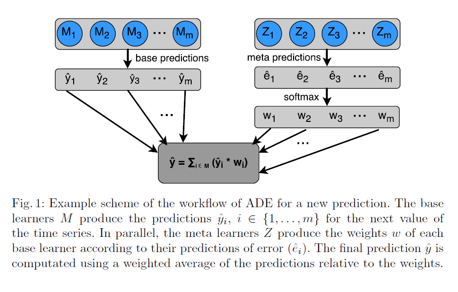
Let us start with this flow chart by the authors of the paper to explain whatever we just described in a nutshell
让我们从论文作者的流程图开始 简而言之解释我们所描述的一切
算法: (The Algorithm:)
(i) Offline-training of M, (the set of base-learners which are used to forecast future values of Y)
(i)M的离线训练(用于预测Y的未来值的一组基础学习器)
(ii) Online-Training or updating of meta-learners Z, which model the expertise of base-learners, and
(ii)对基础学习者的专业知识进行建模的元学习者Z的在线培训或更新,以及
(iii) Online-Prediction of yt+1 using M, dynamically weighed according to Z.
(iii)使用M在线预测yt + 1,并根据Z动态加权。
Important to understand is that the ADE architecture primarily consists of the following:
需要了解的重要一点是,ADE体系结构主要包含以下内容:
i)Base Learners, Mi (Individual, available predictor models)
i)基础学习者,Mi(个人,可用的预测变量模型)
ii)Meta Learners, Zi (Error-tracking models) — 1 per base learner
ii)元学习者Zi(错误跟踪模型)—每个基本学习者1
Given this framework, we are now tasked with determining the meta learner predictions (ei’s in the flowchart). In essence, meta learners Zi are nothing but regression models that aim to predict the error (ei) in base learner predictions (ŷi). This may seem straightforward and logical, but there is one catch.
在此框架下,我们现在的任务是确定元学习者的预测(流程图中的ei)。 本质上,元学习者Zi只是旨在预测基础学习者预测( prediction i)中的误差(ei)的回归模型。 这看似简单明了且合乎逻辑,但有一个陷阱。
With time series, unlike other regression problems, there is the added constraint of temporal dependency and hence, we cannot use any random train-test split to train our models. Note that, for each pocket (window) of time, we need two outputs i) base predictions ŷi and ii) the errors in predictions ei. To obtain (i), we would follow the regular steps that we follow to get univariate time series forecasts (train on a fixed or a walk-forward training window of historical actuals, and forecast on the forecast-horizon window).
与其他回归问题不同,使用时间序列时,存在时间依赖性的附加约束,因此,我们不能使用任何随机训练检验拆分来训练模型。 请注意,对于每个时间段(窗口),我们需要两个输出:i)基本预测ŷi和ii)预测ei的误差。 要获得(i),我们将遵循遵循的常规步骤以获取单变量时间序列预测(在历史实际值的固定或前向训练窗口上进行训练,并在Forecast-horizon窗口上进行预测)。
For getting (ii) though, we need to be ensure that we have our target variable (error in base learner prediction) and training feature matrix engineered correctly. Using some training features, we need to somehowpredict the error in the next time steps before the actuals for those time steps are available themselves (obviously, if we already had the actuals available for the new time steps, what would we even forecast in the first place!) To tackle this problem, the authors propose a simple data transformation/feature engineering exercise on the actuals, called time delay embedding:
为了获得(ii),我们需要确保我们正确设计了目标变量(基本学习者预测中的错误)和训练特征矩阵。 使用一些训练功能,我们需要以某种方式预测下一个时间步长中的错误,然后才能自己获得这些时间步长的实际值(显然,如果我们已经有了新时间步长的实际值,那么我们甚至会在第一个时间步长中预测什么)为了解决这个问题,作者针对实际情况提出了一个简单的数据转换/功能工程练习,称为时间延迟嵌入:
“A time series Y is a temporal sequence of values Y = {y1, y2,….,yt}, where yi is the value of Y at time i. We use time delay embedding to represent Y in an Euclidean space with embedding dimension K. Effectively, we construct a set of observations which are based on the past K lags of the time series. This is accomplished by mapping the time series Y into the embedding vectors
“时间序列Y是值Y = {y1,y2,…。,yt}的时间序列,其中yi是时间i处Y的值。 我们使用时间延迟嵌入来表示具有嵌入维K的欧几里得空间中的Y。有效地,我们基于时间序列的过去K个滞后构造了一组观测值。 这是通过将时间序列Y映射到嵌入向量中来完成的
VN-K+1 = <v1, v2,….,vN-K+1>; where each
VN-K + 1 = <v1,v2,....,vN-K + 1> ; 每个在哪里
vi = <yi-(K-1), yi-(K-2),….yi>.”
vi = <yi-(K-1),yi-(K-2),.... yi> 。”
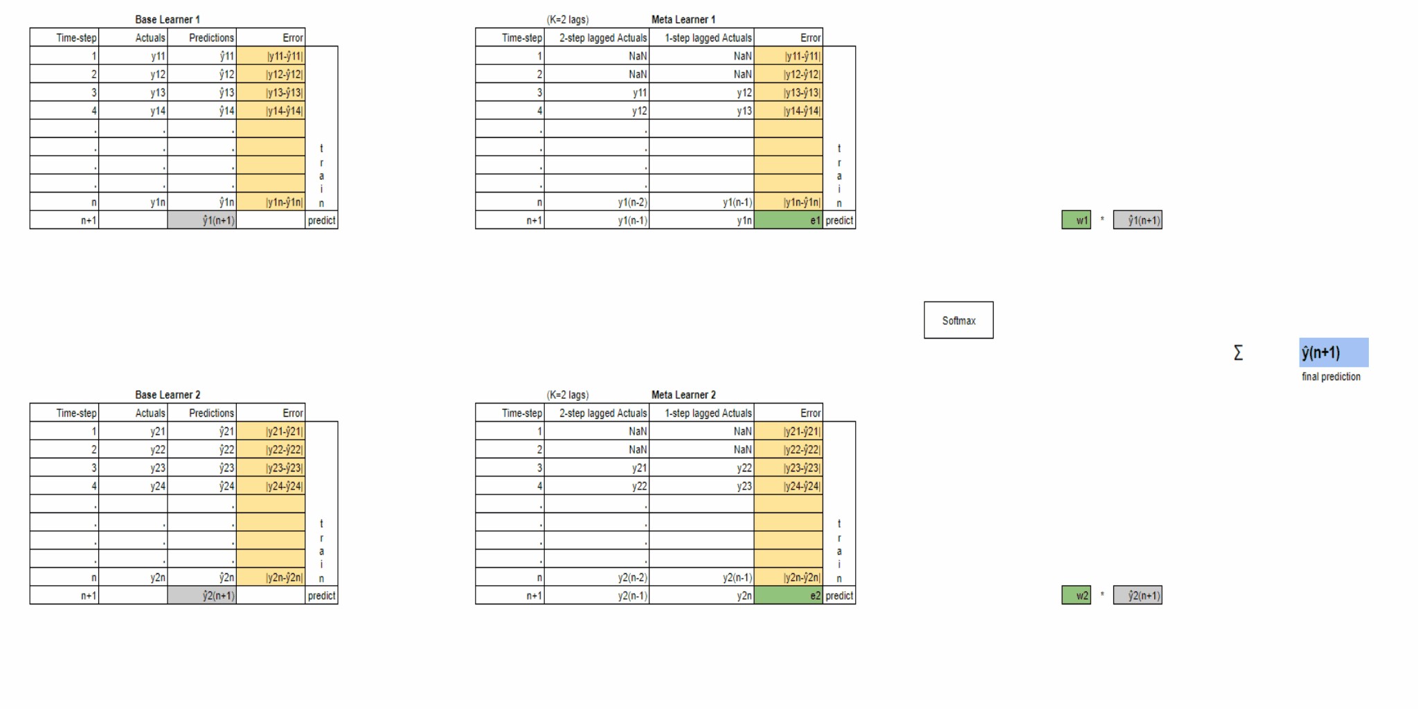
The above animation just visually summarizes the main steps in the ADE algorithm that we’ve previously described already. Note that this animation shows just one iteration of the walk-forward training process. The same sequence of steps will be repeated in the subsequent walk-forward iterations as well, in order to make predictions for upcoming timesteps.
上面的动画只是直观地总结了我们先前已经描述过的ADE算法的主要步骤。 请注意,此动画仅显示前移训练过程的一个迭代。 同样的步骤序列也将在后续的遍历迭代中重复进行,以便对即将到来的时间步进行预测。
Hope this gives you an high-level picture of the working of the ADE model. There are of course, a few more key details that I’ve left out so far that help us tune the performance of the ADE a little better.
希望这能为您提供ADE模型工作的高级概览。 当然,到目前为止,我还遗漏了一些关键细节,这些细节可以帮助我们更好地调整ADE的性能。
1) Weighting Strategy: So far, we’ve only talked about estimating the errors in predictions by the base learners. Notice also, the presence of a SoftMax (of the negative of the error) layer which takes these error estimates as input and returns a probability distribution (array of probabilities adding up to 1). This always scales the errors down to a value between 0 and 1 and makes them easier to compare. By definition, ‘weights’ must add up to 1, so this layer is an ideal choice for computing weights. Note however, that this is not the only way we can approach this. The authors propose an alternative, linear weighting strategy too, one that retains the relative difference between the errors.
1)加权策略:到目前为止,我们仅讨论了基础学习者估计预测中的错误。 还要注意, SoftMax的存在 (误差的负数)层将这些误差估计值作为输入并返回概率分布(概率阵列总计为1)。 这总是将误差缩小到0到1之间的值,并使它们更易于比较。 根据定义,“权重”必须加1,因此该层是计算权重的理想选择。 但是请注意,这不是我们解决此问题的唯一方法。 作者还提出了另一种线性加权策略,该策略保留了误差之间的相对差异。
2) K: We’ve already seen this parameter, that refers to the number of lags to consider to prepare the time-delay embedding vectors as features to train the meta learners Zi. The choice of this parameter will determine how much of recent history to take into account in estimating future error of the base learners.
2) K:我们已经看到了此参数,它是指准备将时间延迟嵌入矢量作为训练元学习者Zi的特征所需考虑的滞后次数。 选择此参数将确定在估计基础学习者的未来错误时要考虑的近期历史记录。
3) Meta Model: So far we’ve only talked about the overall ADE algorithm but not touched upon the choice of the meta learners themselves. Good candidates for meta learners are regression techniques that are themselves ensembles like Gradient Boost, XGBoost and Random Forests. However, meta models can essentially be any other regression model too, like a Linear Regression, but since we’re talking about higher dimensional feature matrices here (time-delay embedding vectors), the formerly mentioned models seem to be better candidates. The authors experiment with multiple different regression models as choices for the meta learners and present their findings in the paper, in case you’re interested.
3)元模型:到目前为止,我们仅讨论了整个ADE算法,但未涉及元学习者自身的选择。 元学习者的很好的候选者是像Gradient Boost , XGBoost和Random Forests这样的集成技术。 但是,元模型在本质上也可以是任何其他回归模型,例如线性回归,但是由于我们在这里谈论的是高维特征矩阵(时间延迟嵌入向量),因此前面提到的模型似乎是更好的候选者。 作者对多种不同的回归模型进行了试验,作为元学习者的选择,并在论文中介绍了他们的发现,以备您感兴趣。
4) Error Metric: This is a crucial factor to consider, for training the meta learners as the errors in the base models are the target vectors for training these meta learners and how exactly these errors are computed and what scale they map to become important considerations. A typical choice is the MAPE (Mean Absolute Percentage Error) as this metric is a relative metric and normalizes the errors down to a percentage value. However, this metric is prone to bias in the case of small actuals. For instance, a prediction of 2 for an actual value of 1 results in a 100% MAPE, which can be misleading at times. A common alternative is the RMSE which is an absolute error and retains the scale of the actuals. However, this metric is prone to scaling issues and it becomes difficult to compare two time series of two different scales using this metric. Common solutions to this problem involve some kind of transformation applied to all the time series in order to first normalize them to a comparable scale.
4)错误度量:对于训练元学习者,这是要考虑的关键因素,因为基本模型中的错误是训练这些元学习者的目标向量,以及如何精确计算这些错误以及将其映射为何种比例成为重要考虑因素。 典型的选择是MAPE (平均绝对百分比误差),因为此度量是相对度量,并且将误差归一化为百分比值。 但是,在实际数据较少的情况下,此指标容易产生偏差。 例如,对于实际值为1的2预测会导致100%MAPE,这有时可能会引起误解。 常见的替代方法是RMSE ,它是绝对误差,并且保留实际值的大小。 但是,此度量标准容易出现缩放问题,并且使用此度量标准来比较两个不同尺度的两个时间序列变得很困难。 这个问题的常见解决方案包括对所有时间序列进行某种转换,以便首先将它们标准化为可比较的标度。
The parameters discussed so far concern a single iteration of the walk-forward. The last two parameters that we will talk about however, are related to a key idea that spans all iterations, which we discussed in the introduction of this article — an individual base learner cannot be practically expected to perform consistently well throughout the time series. Hence, the notion of leveraging localized expertise of some models in some regions of time and others during other regions of time. The authors thus, introduce two more parameters that are used to filter out the non-expert base models for that region of time. 5) Omega: This is just the length of time in recent history to consider for evaluating the average error metric of all base models on, so that the models with the worst averages, can be discarded from this ‘committee’ of models.6) Alpha: This is the number of top base models to consider in the ‘committee’ of models that then have a say in the combined forecast for the given timestep
到目前为止讨论的参数涉及前移的单个迭代。 但是,我们将要讨论的最后两个参数与跨越所有迭代的关键思想有关,我们在本文的简介中讨论了这一思想-实际上,不能期望单个基础学习者在整个时间序列中都能始终如一地表现良好。 因此,在某些时间区域中利用某些模型的本地化专业知识,而在其他时间区域中利用其他模型的概念。 因此,作者引入了另外两个参数,用于过滤该时间段内的非专家基础模型。 5)欧米茄(Omega):这只是近期历史,可以用来评估所有基础模型的平均误差度量,因此可以从该模型的“委员会”中丢弃平均值最差的模型。6) Alpha:这是模型“委员会”中要考虑的顶级基础模型的数量,然后这些模型在给定时间步长的组合预测中具有发言权
结语!(Wrapping Up!)
Hopefully, this has given you enough of a conceptual and a mathematical intuition around the motivations behind the Arbitrated Dynamic Ensemble Model to try it out yourself! Of course there are several other things one can experiment with like normalization, feature-engineering and what not! The purpose of this article was just to give you a quick primer on a novel ensemble technique that is specialized for time series forecasting problems, but if you’re interested in more of the geeky stuff, I’d highly recommend giving the original paper a read. Trust me, it will be worth your time!
希望这为您提供了足够的概念性和数学直觉,可以帮助他们了解仲裁动态集成模型背后的动机! 当然,还有其他一些可以尝试的东西,例如规范化,功能工程以及其他不能尝试的东西! 本文的目的只是为您提供一种专门针对时间序列预测问题的新颖合奏技术的快速入门,但是,如果您对更多令人讨厌的东西感兴趣,我强烈建议您给原始论文一个读。 相信我,这将是您的宝贵时间!
But what’s a technique without a word on its applications, right? Let me quickly talk about why and how I have used this model. Unfortunately, due to company policies around restrictions of data privacy, I am unable to show real data here. Nonetheless, the results represent the real outcomes, just with dummy labels.
但是,什么是应用程序却一言不发的技术呢? 让我快速谈谈为什么以及如何使用此模型。 不幸的是,由于公司有关数据隐私限制的政策,我无法在此处显示真实数据。 尽管如此,仅使用虚拟标签,结果仍代表实际结果。
A quick background on the problem statement: I work for a team that helps support 40+ operational teams plan their resources so that they are better able to handle incoming demand. My role is to generate demand forecasts for each of these operational teams. We have a suite of models that we’ve developed ranging from Simple Moving Averages to ARIMA to Exponential Smoothing Models. However, the challenge lies in the varied nature of these different teams. No single model does well for all teams, and also even for a given team, no single model does well for the entire length of the time series, which in our case, is close to 4 years — because at different points in time, many of the the teams exhibit dynamic trends and seasonality. That’s when I stumbled upon this paper and thus, the adventure began!
问题陈述的快速背景:我为一个团队工作,该团队帮助支持40多个运营团队计划其资源,以便他们能够更好地处理传入的需求。 我的职责是为每个运营团队生成需求预测。 我们开发了一系列模型,从简单移动平均线到ARIMA到指数平滑模型。 但是,挑战在于这些不同团队的多样性。 没有一个单一的模型对所有团队都适用,甚至对于一个给定的团队,也没有一个单一的模型在整个时间序列的长度上都表现良好,在我们的案例中,这接近4年-因为在不同的时间点,其中的团队表现出动态变化和季节变化。 那是我偶然发现本文的时候,冒险开始了!
Below are sample results from some experiments (with different choices of weight layer and alpha) run on one of the teams. Notice that in all three of these experiments, the ADE performs the best in terms of MAPE as compared to the other top 4 base models. (The ADE’s MAPE is better than the MAPE of the best base learner model by about 2% points, which is quite significant, given the range of the RMSEs) The meta model used here was fixed to a GBM model.
以下是其中一个小组进行的一些实验(使用不同的权重层和alpha选择)的示例结果。 请注意,在所有这三个实验中,相对于其他前4个基本模型,ADE在MAPE方面表现最佳。 (ADE的MAPE比最佳基础学习者模型的MAPE好2%点,考虑到RMSE的范围,这是非常重要的。)这里使用的元模型固定为GBM模型。
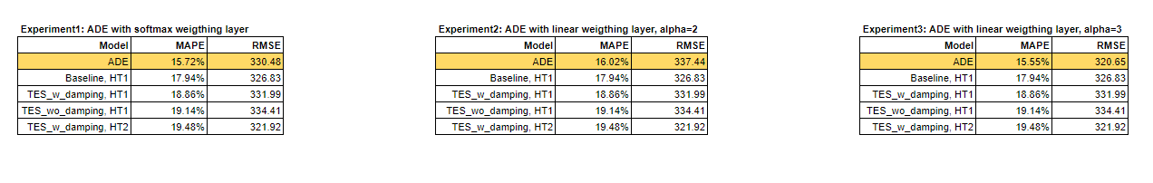
It can be tempting to draw generalized conclusions from such results about the best choice of hyperparameters like weighting strategy and alpha, but its important to realize that what may work best for one team (one time series), might not necessarily hold good for another. In such a situation, hyperparameter tuning methods like gridsearch come in quite handy. Considering also the fact that other than the 6 parameters (or degrees of freedom) defined above, we also have the meta-model’s own set of hyperparameters that we can tune, this would scale up the number of possible combinations and thus the model training time, exponentially. A parallelized version of gridsearch using spark RDDs could come in handy, as described in this Databricks blog.
从这样的结果中得出关于最佳选择超参数(如加权策略和alpha)的概括性结论可能很诱人,但重要的是要认识到什么可能对一个团队(一个时间序列)最有效,不一定对另一个团队有利。 在这种情况下,诸如网格搜索之类的超参数调整方法非常方便。 还考虑以下事实,除了上面定义的6个参数(或自由度),我们还有元模型自己可以调整的超参数集,这将扩大可能组合的数量,从而增加模型训练时间,呈指数增长。 如本Databricks博客所述,使用Spark RDD的并行并行版本的gridsearch可能会派上用场。
The point is, there are a lot of different cogs to this machine and the best combination really depends on the data being modelled and the available set of base learner models, so don’t be afraid to experiment!
关键是,这台机器有很多不同的齿轮,最佳组合的确取决于建模数据和可用的基础学习者模型集,因此不要害怕进行试验!
For those of you who are R users, the authors of the paper have released an R package for this model called tsensembler.
对于那些使用R的用户,本文的作者发布了针对该模型的R软件包tsensembler 。
We however, built our code from scratch in python as the rest of our base models and the main code base were already in python. This however, gave us some flexibility to generalize our version of the ADE to work with any choice of base models, unlike the R package which limits the available base models to a only a few. Unfortunately, I am unable to share any of my code here, but the fact that I could code up a basic version of the ADE from scratch by reading the paper should be motivation enough for you to put on your solution-designer hats and get going! If at all you are stuck somewhere, I am more than happy to help out where I can — just drop in a comment here!
但是,我们的其余基本模型和主要代码库已经在python中,因此我们从头开始在python中构建了代码。 但是,这给了我们一定的灵活性,使我们的ADE版本可以与任何基本模型选择一起使用,而不像R软件包那样将可用的基本模型限制为仅几个。 不幸的是,我无法在此处共享我的任何代码,但事实上,我可以通过阅读本文从头开始编写ADE的基本版本,这足以激励您穿上解决方案设计师的帽子,并继续前进! 如果您完全被困在某个地方,我很乐意在可能的地方提供帮助-请在此处发表评论!
A word of advice-your ADE can only do as well as the best of your base learner models (its their weighted average), so its still essential to focus your attention on improving the performances of those individual models first! Also, it remains to be seen how well the ADE performs with multivariate time series problems — we’ve so far, tried it only on univariate base learner models.
一言以蔽之,您的ADE只能与您的基础学习模型中最好的(它的加权平均)一样好,因此仍然必须首先集中精力改善单个模型的性能! 此外,还有待观察ADE在多元时间序列问题上的表现如何-到目前为止,我们仅在单变量基础学习器模型上进行过尝试。
The authors experimented with this model on several kinds of datasets and forecasting problems ranging from Energy Demand Forecasting, Solar Radiation Forecasting and Ozone Level Detection. This should give an indication of the robustness of this algorithm across several domains!
作者在多种数据集和预测问题(包括能源需求预测,太阳辐射预测和臭氧水平检测)上对该模型进行了试验。 这应该表明该算法在多个域中的鲁棒性!
Finally though, a philosophical note to wrap things up! The reason why I find the ADE so beautiful, is because of the parallels I am able to draw with life — my own, in particular. I am a jack of several trades (and I’d like to think, a master of some!) I enjoy drumming and singing on some days. On others, I turn to creating short animation films. On other days still, I simply like to jot down my thoughts. Point is, I find it really hard to continue doing tomorrow what I enjoyed doing today — that’s just who I am. But realizing this fact itself, gives me peace — that I need to do what’s really right for that moment — leverage localized expertise!
最后,尽管如此,但还是用哲学的手法总结了一下! 我之所以认为ADE如此漂亮,是因为我能够与生活相提并论,尤其是我自己。 我是几个行业的杰克(我想想,是一些大师!)我喜欢在某些日子里鼓和唱歌。 在其他方面,我转向制作动画短片。 还有几天,我只是想记一下我的想法。 关键是,我发现很难继续明天做我今天喜欢做的事情-那就是我。 但是,认识到这一事实本身,就可以给我带来和平-我需要做那时候真正正确的事情-利用本地化的专业知识!
Follow me on my LinkedIn profile or leave a comment here, and I’d be happy to respond!
在我的LinkedIn个人资料上关注我,或在这里发表评论,我很乐意回应!


 被折叠的 条评论
为什么被折叠?
被折叠的 条评论
为什么被折叠?
 到【灌水乐园】发言


