


【机器学习练习 5】 - 偏差和方差的权衡
本章代码涵盖了基于Python的解决方案,用于Coursera机器学习课程的第五个编程练习。
数据集链接 链接
import numpy as np
import scipy.io as sio
import scipy.optimize as opt
import pandas as pd
import matplotlib.pyplot as plt
import seaborn as sns
def load_data():
    """for ex5
    d['X'] shape = (12, 1)
    pandas has trouble taking this 2d ndarray to construct a dataframe, so I ravel
    the results
    """
    d = sio.loadmat('ex5data1.mat')
    return map(np.ravel, [d['X'], d['y'], d['Xval'], d['yval'], d['Xtest'], d['ytest']])
X, y, Xval, yval, Xtest, ytest = load_data()
X, y, Xval, yval, Xtest, ytest
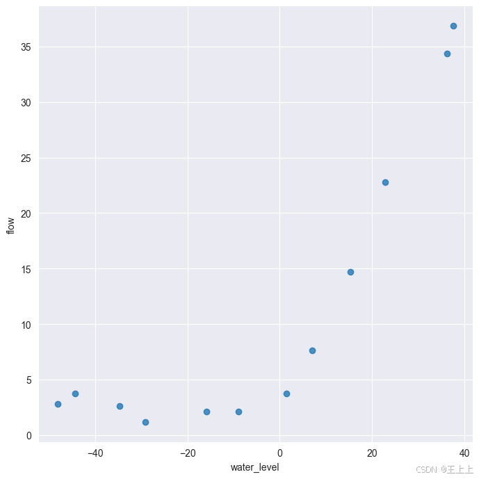
df = pd.DataFrame({'water_level':X, 'flow':y})

sns.lmplot(x='water_level', y='flow', data=df, fit_reg=False, height=7)
plt.show()
X, Xval, Xtest = [np.insert(x.reshape(x.shape[0], 1), 0, np.ones(x.shape[0]), axis=1) for x in (X, Xval, Xtest)]
代价函数
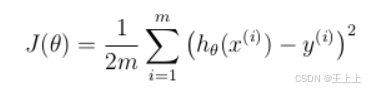
def cost(theta, X, y):
    """
    X: R(m*n), m records, n features
    y: R(m)
    theta : R(n), linear regression parameters
    """
    m = X.shape[0]

    inner = X @ theta - y  # R(m*1)

    # 1*m @ m*1 = 1*1 in matrix multiplication
    # but you know numpy didn't do transpose in 1d array, so here is just a
    # vector inner product to itselves
    square_sum = inner.T @ inner
    cost = square_sum / (2 * m)

    return cost
theta = np.ones(X.shape[1])
cost(theta, X, y)
303.95152555359766
梯度
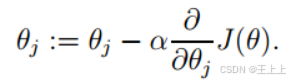
def gradient(theta, X, y):
    m = X.shape[0]

    inner = X.T @ (X @ theta - y)  # (m,n).T @ (m, 1) -> (n, 1)

    return inner / m
gradient(theta, X, y)
array([-15.30301567, 598.16741084])
正则化梯度
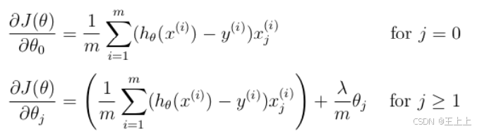
def regularized_gradient(theta, X, y, l=1):
    m = X.shape[0]

    regularized_term = theta.copy()  # same shape as theta
    regularized_term[0] = 0  # don't regularize intercept theta

    regularized_term = (l / m) * regularized_term

    return gradient(theta, X, y) + regularized_term
regularized_gradient(theta, X, y)
array([-15.30301567, 598.25074417])
拟合数据
正则化项 λ = 0 \lambda=0 λ=0
def linear_regression_np(X, y, l=1):
    """linear regression
    args:
        X: feature matrix, (m, n+1) # with incercept x0=1
        y: target vector, (m, )
        l: lambda constant for regularization

    return: trained parameters
    """
    # init theta
    theta = np.ones(X.shape[1])

    # train it
    res = opt.minimize(fun=regularized_cost,
                       x0=theta,
                       args=(X, y, l),
                       method='TNC',
                       jac=regularized_gradient,
                       options={'disp': True})
    return res
def regularized_cost(theta, X, y, l=1):
    m = X.shape[0]

    regularized_term = (l / (2 * m)) * np.power(theta[1:], 2).sum()

    return cost(theta, X, y) + regularized_term
theta = np.ones(X.shape[0])

final_theta = linear_regression_np(X, y, l=0).get('x')
b = final_theta[0] # intercept
m = final_theta[1] # slope
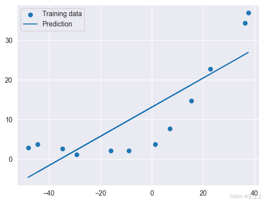
plt.scatter(X[:,1], y, label="Training data")
plt.plot(X[:, 1], X[:, 1]*m + b, label="Prediction")
plt.legend(loc=2)
plt.show()
training_cost, cv_cost = [], []
1.使用训练集的子集来拟合应模型
2.在计算训练代价和交叉验证代价时,没有用正则化
3.记住使用相同的训练集子集来计算训练代价
m = X.shape[0]
for i in range(1, m+1):
#     print('i={}'.format(i))
    res = linear_regression_np(X[:i, :], y[:i], l=0)

    tc = regularized_cost(res.x, X[:i, :], y[:i], l=0)
    cv = regularized_cost(res.x, Xval, yval, l=0)
#     print('tc={}, cv={}'.format(tc, cv))

    training_cost.append(tc)
    cv_cost.append(cv)
plt.plot(np.arange(1, m+1), training_cost, label='training cost')
plt.plot(np.arange(1, m+1), cv_cost, label='cv cost')
plt.legend(loc=1)
plt.show()
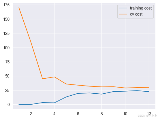
这个模型拟合不太好, 欠拟合了
创建多项式特征
def prepare_poly_data(*args, power):
    """
    args: keep feeding in X, Xval, or Xtest
        will return in the same order
    """
    def prepare(x):
        # expand feature
        df = poly_features(x, power=power)

        # normalization
        ndarr = normalize_feature(df).as_matrix()

        # add intercept term
        return np.insert(ndarr, 0, np.ones(ndarr.shape[0]), axis=1)

    return [prepare(x) for x in args]
def poly_features(x, power, as_ndarray=False):
    data = {'f{}'.format(i): np.power(x, i) for i in range(1, power + 1)}
    df = pd.DataFrame(data)

    return df.as_matrix() if as_ndarray else df
X, y, Xval, yval, Xtest, ytest = load_data()
poly_features(X, power=3)
| f1 | f2 | f3 | |
|---|---|---|---|
| 0 | -15.936758 | 253.980260 | -4047.621971 |
| 1 | -29.152979 | 849.896197 | -24777.006175 |
| 2 | 36.189549 | 1309.683430 | 47396.852168 |
| 3 | 37.492187 | 1405.664111 | 52701.422173 |
| 4 | -48.058829 | 2309.651088 | -110999.127750 |
| 5 | -8.941458 | 79.949670 | -714.866612 |
| 6 | 15.307793 | 234.328523 | 3587.052500 |
| 7 | -34.706266 | 1204.524887 | -41804.560890 |
| 8 | 1.389154 | 1.929750 | 2.680720 |
| 9 | -44.383760 | 1969.918139 | -87432.373590 |
| 10 | 7.013502 | 49.189211 | 344.988637 |
| 11 | 22.762749 | 518.142738 | 11794.353058 |
准备多项式回归数据
- 扩展特征到 8阶,或者你需要的阶数
- 使用 归一化 来合并 x n x^n xn
- don’t forget intercept term
def normalize_feature(df):
    """Applies function along input axis(default 0) of DataFrame."""
    return df.apply(lambda column: (column - column.mean()) / column.std())
def prepare_poly_data(*args, power):
    """
    args: keep feeding in X, Xval, or Xtest
        will return in the same order
    """
    def prepare(x):
        # expand feature
        df = poly_features(x, power=power)

        # normalization
        ndarr = normalize_feature(df).to_numpy()  # 修改这里

        # add intercept term
        return np.insert(ndarr, 0, np.ones(ndarr.shape[0]), axis=1)

    return [prepare(x) for x in args]

X_poly, Xval_poly, Xtest_poly = prepare_poly_data(X, Xval, Xtest, power=8)
X_poly[:3, :]
array([[ 1.00000000e+00, -3.62140776e-01, -7.55086688e-01,
         1.82225876e-01, -7.06189908e-01,  3.06617917e-01,
        -5.90877673e-01,  3.44515797e-01, -5.08481165e-01],
       [ 1.00000000e+00, -8.03204845e-01,  1.25825266e-03,
        -2.47936991e-01, -3.27023420e-01,  9.33963187e-02,
        -4.35817606e-01,  2.55416116e-01, -4.48912493e-01],
       [ 1.00000000e+00,  1.37746700e+00,  5.84826715e-01,
         1.24976856e+00,  2.45311974e-01,  9.78359696e-01,
        -1.21556976e-02,  7.56568484e-01, -1.70352114e-01]])
表格:前 3 行的多项式扩展特征
| Feature Index | x 1 1 x 2 0 x_1^1 x_2^0 x11x20 (F10) | x 1 2 x 2 0 x_1^2 x_2^0 x12x20 (F20) | x 1 3 x 2 0 x_1^3 x_2^0 x13x20 (F30) | x 1 4 x 2 0 x_1^4 x_2^0 x14x20 (F40) | x 1 5 x 2 0 x_1^5 x_2^0 x15x20 (F50) | x 1 1 x 2 1 x_1^1 x_2^1 x11x21 (F11) | x 1 2 x 2 1 x_1^2 x_2^1 x12x21 (F21) | x 1 3 x 2 1 x_1^3 x_2^1 x13x21 (F31) | x 1 4 x 2 1 x_1^4 x_2^1 x14x21 (F41) | x 1 5 x 2 1 x_1^5 x_2^1 x15x21 (F51) | x 1 1 x 2 2 x_1^1 x_2^2 x11x22 (F12) | x 1 2 x 2 2 x_1^2 x_2^2 x12x22 (F22) | x 1 3 x 2 2 x_1^3 x_2^2 x13x22 (F32) | x 1 4 x 2 2 x_1^4 x_2^2 x14x22 (F42) | x 1 5 x 2 2 x_1^5 x_2^2 x15x22 (F52) | x 1 1 x 2 3 x_1^1 x_2^3 x11x23 (F13) | x 1 2 x 2 3 x_1^2 x_2^3 x12x23 (F23) | x 1 3 x 2 3 x_1^3 x_2^3 x13x23 (F33) | x 1 4 x 2 3 x_1^4 x_2^3 x14x23 (F43) | x 1 5 x 2 3 x_1^5 x_2^3 x15x23 (F53) | x 1 1 x 2 4 x_1^1 x_2^4 x11x24 (F14) | x 1 2 x 2 4 x_1^2 x_2^4 x12x24 (F24) | x 1 3 x 2 4 x_1^3 x_2^4 x13x24 (F34) | x 1 4 x 2 4 x_1^4 x_2^4 x14x24 (F44) | x 1 5 x 2 4 x_1^5 x_2^4 x15x24 (F54) |
|---|---|---|---|---|---|---|---|---|---|---|---|---|---|---|---|---|---|---|---|---|---|---|---|---|---|
| 0 | x 1 1 x 2 0 x_1^1 x_2^0 x11x20 | x 1 2 x 2 0 x_1^2 x_2^0 x12x20 | x 1 3 x 2 0 x_1^3 x_2^0 x13x20 | x 1 4 x 2 0 x_1^4 x_2^0 x14x20 | x 1 5 x 2 0 x_1^5 x_2^0 x15x20 | x 1 1 x 2 1 x_1^1 x_2^1 x11x21 | x 1 2 x 2 1 x_1^2 x_2^1 x12x21 | x 1 3 x 2 1 x_1^3 x_2^1 x13x21 | x 1 4 x 2 1 x_1^4 x_2^1 x14x21 | x 1 5 x 2 1 x_1^5 x_2^1 x15x21 | x 1 1 x 2 2 x_1^1 x_2^2 x11x22 | x 1 2 x 2 2 x_1^2 x_2^2 x12x22 | x 1 3 x 2 2 x_1^3 x_2^2 x13x22 | x 1 4 x 2 2 x_1^4 x_2^2 x14x22 | x 1 5 x 2 2 x_1^5 x_2^2 x15x22 | x 1 1 x 2 3 x_1^1 x_2^3 x11x23 | x 1 2 x 2 3 x_1^2 x_2^3 x12x23 | x 1 3 x 2 3 x_1^3 x_2^3 x13x23 | x 1 4 x 2 3 x_1^4 x_2^3 x14x23 | x 1 5 x 2 3 x_1^5 x_2^3 x15x23 | x 1 1 x 2 4 x_1^1 x_2^4 x11x24 | x 1 2 x 2 4 x_1^2 x_2^4 x12x24 | x 1 3 x 2 4 x_1^3 x_2^4 x13x24 | x 1 4 x 2 4 x_1^4 x_2^4 x14x24 | x 1 5 x 2 4 x_1^5 x_2^4 x15x24 |
| 1 | x 1 1 x 2 0 x_1^1 x_2^0 x11x20 | x 1 2 x 2 0 x_1^2 x_2^0 x12x20 | x 1 3 x 2 0 x_1^3 x_2^0 x13x20 | x 1 4 x 2 0 x_1^4 x_2^0 x14x20 | x 1 5 x 2 0 x_1^5 x_2^0 x15x20 | x 1 1 x 2 1 x_1^1 x_2^1 x11x21 | x 1 2 x 2 1 x_1^2 x_2^1 x12x21 | x 1 3 x 2 1 x_1^3 x_2^1 x13x21 | x 1 4 x 2 1 x_1^4 x_2^1 x14x21 | x 1 5 x 2 1 x_1^5 x_2^1 x15x21 | x 1 1 x 2 2 x_1^1 x_2^2 x11x22 | x 1 2 x 2 2 x_1^2 x_2^2 x12x22 | x 1 3 x 2 2 x_1^3 x_2^2 x13x22 | x 1 4 x 2 2 x_1^4 x_2^2 x14x22 | x 1 5 x 2 2 x_1^5 x_2^2 x15x22 | x 1 1 x 2 3 x_1^1 x_2^3 x11x23 | x 1 2 x 2 3 x_1^2 x_2^3 x12x23 | x 1 3 x 2 3 x_1^3 x_2^3 x13x23 | x 1 4 x 2 3 x_1^4 x_2^3 x14x23 | x 1 5 x 2 3 x_1^5 x_2^3 x15x23 | x 1 1 x 2 4 x_1^1 x_2^4 x11x24 | x 1 2 x 2 4 x_1^2 x_2^4 x12x24 | x 1 3 x 2 4 x_1^3 x_2^4 x13x24 | x 1 4 x 2 4 x_1^4 x_2^4 x14x24 | x 1 5 x 2 4 x_1^5 x_2^4 x15x24 |
| 2 | x 1 1 x 2 0 x_1^1 x_2^0 x11x20 | x 1 2 x 2 0 x_1^2 x_2^0 x12x20 | x 1 3 x 2 0 x_1^3 x_2^0 x13x20 | x 1 4 x 2 0 x_1^4 x_2^0 x14x20 | x 1 5 x 2 0 x_1^5 x_2^0 x15x20 | x 1 1 x 2 1 x_1^1 x_2^1 x11x21 | x 1 2 x 2 1 x_1^2 x_2^1 x12x21 | x 1 3 x 2 1 x_1^3 x_2^1 x13x21 | x 1 4 x 2 1 x_1^4 x_2^1 x14x21 | x 1 5 x 2 1 x_1^5 x_2^1 x15x21 | x 1 1 x 2 2 x_1^1 x_2^2 x11x22 | x 1 2 x 2 2 x_1^2 x_2^2 x12x22 | x 1 3 x 2 2 x_1^3 x_2^2 x13x22 | x 1 4 x 2 2 x_1^4 x_2^2 x14x22 | x 1 5 x 2 2 x_1^5 x_2^2 x15x22 | x 1 1 x 2 3 x_1^1 x_2^3 x11x23 | x 1 2 x 2 3 x_1^2 x_2^3 x12x23 | x 1 3 x 2 3 x_1^3 x_2^3 x13x23 | x 1 4 x 2 3 x_1^4 x_2^3 x14x23 | x 1 5 x 2 3 x_1^5 x_2^3 x15x23 | x 1 1 x 2 4 x_1^1 x_2^4 x11x24 | x 1 2 x 2 4 x_1^2 x_2^4 x12x24 | x 1 3 x 2 4 x_1^3 x_2^4 x13x24 | x 1 4 x 2 4 x_1^4 x_2^4 x14x24 | x 1 5 x 2 4 x_1^5 x_2^4 x15x24 |
说明:
- F10, F20, F30, … 是各个特征的编号,表示每一列是
x1和x2的组合。 x1^1 x2^0表示x1的 1 次幂,x2的 0 次幂,即x1本身。x1^2 x2^1表示x1的 2 次幂和x2的 1 次幂,即x1^2 * x2。- 继续按照这个规则,特征的组合会逐步从低次幂扩展到高次幂,直到 8 次幂为止。
如果你已经将 X_poly 等数据转化为多项式特征,前三行数据将呈现类似的格式。
画出学习曲线
首先,我们没有使用正则化,所以 λ = 0 \lambda=0 λ=0
def plot_learning_curve(X, y, Xval, yval, l=0):
    training_cost, cv_cost = [], []
    m = X.shape[0]

    for i in range(1, m + 1):
        # regularization applies here for fitting parameters
        res = linear_regression_np(X[:i, :], y[:i], l=l)

        # remember, when you compute the cost here, you are computing
        # non-regularized cost. Regularization is used to fit parameters only
        tc = cost(res.x, X[:i, :], y[:i])
        cv = cost(res.x, Xval, yval)

        training_cost.append(tc)
        cv_cost.append(cv)

    plt.plot(np.arange(1, m + 1), training_cost, label='training cost')
    plt.plot(np.arange(1, m + 1), cv_cost, label='cv cost')
    plt.legend(loc=1)
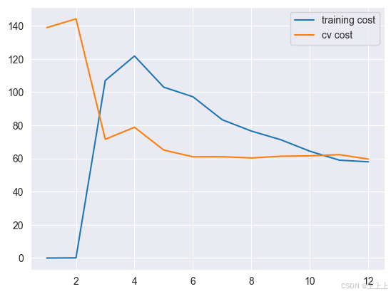
plot_learning_curve(X_poly, y, Xval_poly, yval, l=0)
plt.show()
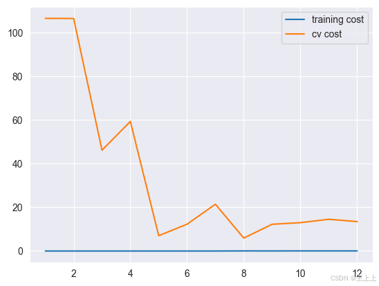
你可以看到训练的代价太低了,不真实. 这是 过拟合了
try λ = 1 \lambda=1 λ=1
plot_learning_curve(X_poly, y, Xval_poly, yval, l=1)
plt.show()
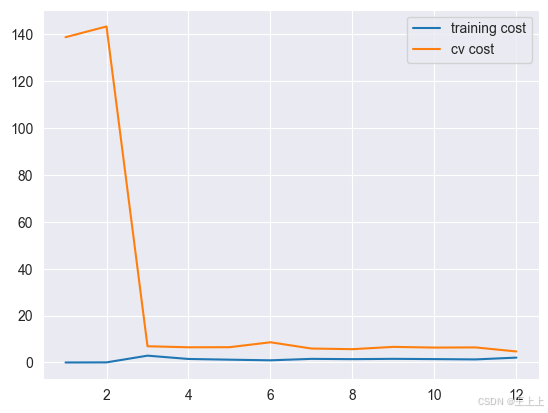
训练代价增加了些,不再是0了。
也就是说我们减轻过拟合
try λ = 100 \lambda=100 λ=100
plot_learning_curve(X_poly, y, Xval_poly, yval, l=100)
plt.show()
太多正则化了.
变成 欠拟合状态
找到最佳的 λ \lambda λ
l_candidate = [0, 0.001, 0.003, 0.01, 0.03, 0.1, 0.3, 1, 3, 10]
training_cost, cv_cost = [], []
for l in l_candidate:
    res = linear_regression_np(X_poly, y, l)

    tc = cost(res.x, X_poly, y)
    cv = cost(res.x, Xval_poly, yval)

    training_cost.append(tc)
    cv_cost.append(cv)
plt.plot(l_candidate, training_cost, label='training')
plt.plot(l_candidate, cv_cost, label='cross validation')
plt.legend(loc=2)

plt.xlabel('lambda')

plt.ylabel('cost')
plt.show()
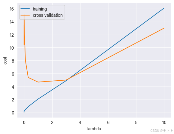
# best cv I got from all those candidates
l_candidate[np.argmin(cv_cost)]
1
# use test data to compute the cost
cost_results = {}

for l in l_candidate:
    theta = linear_regression_np(X_poly, y, l).x
    test_cost = cost(theta, Xtest_poly, ytest)
    cost_results[l] = test_cost
    print(f'test cost(l={l}) = {test_cost}')

# 找到最小的 test cost 对应的 l
best_l = min(cost_results, key=cost_results.get)
print(f'最小的 test cost 对应的 λ = {best_l}, cost = {cost_results[best_l]}')
test cost(l=0) = 10.02464287753563
test cost(l=0.001) = 11.03989643825398
test cost(l=0.003) = 11.263612931846453
test cost(l=0.01) = 10.87954944353898
test cost(l=0.03) = 10.022095688423208
test cost(l=0.1) = 8.632065168219597
test cost(l=0.3) = 7.336723122820889
test cost(l=1) = 7.466289574046468
test cost(l=3) = 11.643928179962794
test cost(l=10) = 27.715080206181412
最小的 test cost 对应的 λ = 0.3, cost = 7.336723122820889
调参后, λ = 0.3 \lambda = 0.3 λ=0.3 是最优选择,这个时候测试代价最小


 1981
1981

 被折叠的 条评论
为什么被折叠?
被折叠的 条评论
为什么被折叠?
 到【灌水乐园】发言


