吴恩达《Machine Learning》-machine-learning-ex4神经网络学习作业（四）

nnCostFunction.m

对于神经网络我们需要计算其损失函数值J(θ)与grad梯度。
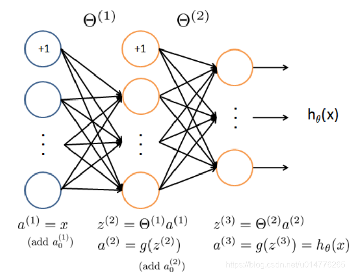
1.前向传播计算损失函数值J(θ)
首先计算hθ（x）=a（3）
公式如下：

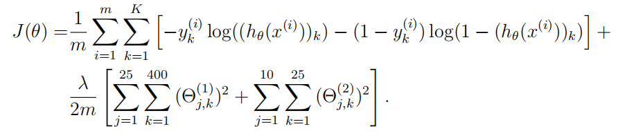
加入正则项的损失函数公式（注意程序中为向量表达，此处为数值表达）：

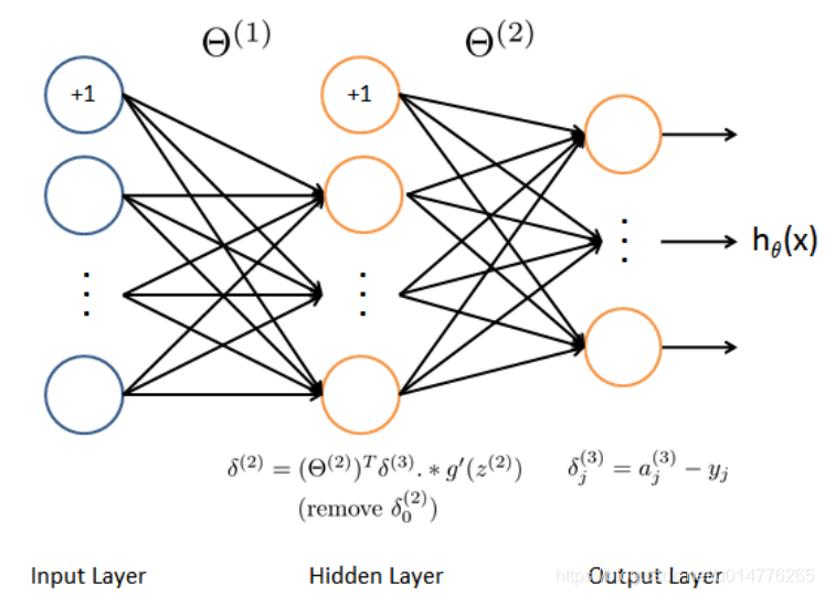
2.反向传播计算梯度grad
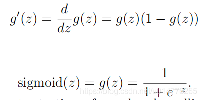
公式中使用了g^’(z⁽²⁾)，故应先实现sigmod梯度值函数sigmoidGradient(z)。
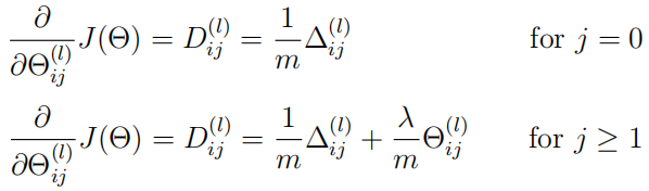
之后按照公式计算：

grad梯度计算：

function [J grad] = nnCostFunction(nn_params, ...
                                   input_layer_size, ...
                                   hidden_layer_size, ...
                                   num_labels, ...
                                   X, y, lambda)
%NNCOSTFUNCTION Implements the neural network cost function for a two layer
%neural network which performs classification
%   [J grad] = NNCOSTFUNCTON(nn_params, hidden_layer_size, num_labels, ...
%   X, y, lambda) computes the cost and gradient of the neural network. The
%   parameters for the neural network are "unrolled" into the vector
%   nn_params and need to be converted back into the weight matrices. 
% 
%   The returned parameter grad should be a "unrolled" vector of the
%   partial derivatives of the neural network.
%

% Reshape nn_params back into the parameters Theta1 and Theta2, the weight matrices
% for our 2 layer neural network
Theta1 = reshape(nn_params(1:hidden_layer_size * (input_layer_size + 1)), ...
                 hidden_layer_size, (input_layer_size + 1));

Theta2 = reshape(nn_params((1 + (hidden_layer_size * (input_layer_size + 1))):end), ...
                 num_labels, (hidden_layer_size + 1));

% Setup some useful variables
m = size(X, 1);
         
% You need to return the following variables correctly 
J = 0;
Theta1_grad = zeros(size(Theta1));
Theta2_grad = zeros(size(Theta2));

% ====================== YOUR CODE HERE ======================
% Instructions: You should complete the code by working through the
%               following parts.
%
% Part 1: Feedforward the neural network and return the cost in the
%         variable J. After implementing Part 1, you can verify that your
%         cost function computation is correct by verifying the cost
%         computed in ex4.m
%
% Part 2: Implement the backpropagation algorithm to compute the gradients
%         Theta1_grad and Theta2_grad. You should return the partial derivatives of
%         the cost function with respect to Theta1 and Theta2 in Theta1_grad and
%         Theta2_grad, respectively. After implementing Part 2, you can check
%         that your implementation is correct by running checkNNGradients
%
%         Note: The vector y passed into the function is a vector of labels
%               containing values from 1..K. You need to map this vector into a 
%               binary vector of 1's and 0's to be used with the neural network
%               cost function.
%
%         Hint: We recommend implementing backpropagation using a for-loop
%               over the training examples if you are implementing it for the 
%               first time.
%
% Part 3: Implement regularization with the cost function and gradients.
%
%         Hint: You can implement this around the code for
%               backpropagation. That is, you can compute the gradients for
%               the regularization separately and then add them to Theta1_grad
%               and Theta2_grad from Part 2.
%

temp = zeros(m,num_labels);
for j = 1:size(y,1)
temp(j,y(j)) = 1;
endfor
y = temp;
X = [ones(m,1) X];

%前向传播计算J
a2 = sigmoid(X * Theta1');
a3 = sigmoid([ones(size(a2,1),1) a2] * Theta2');
J = 1/m * sum(sum((-y).*log(a3) - (1-y).*log(1-a3)))+ lambda/(2*m)*...
(sum(sum(Theta1(:,2:input_layer_size+1).^2)) + sum(sum(Theta2(:,2:hidden_layer_size+1).^2)));
 
%反向传播计算grad
Error_3 = a3 - y;
sigmoidgrad1 = sigmoidGradient(X * Theta1');
Error_2 = Error_3 * Theta2  .* [ones(size(sigmoidgrad1,1),1) sigmoidgrad1];
Theta1_grad =1/m * Error_2(:,2:end)' * X + lambda/m * [zeros(size(Theta1,1),1)  Theta1(:,2:end)];
Theta2_grad =1/m * Error_3' * [ones(size(a2,1),1) a2] + lambda/m * [zeros(size(Theta2,1),1)  Theta2(:,2:end)];



% -------------------------------------------------------------

% =========================================================================

% Unroll gradients
grad = [Theta1_grad(:) ; Theta2_grad(:)];


end

运行结果

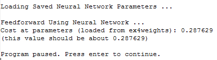
前向传播损失值J：

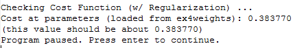
前向传播加入正则化的损失值J：

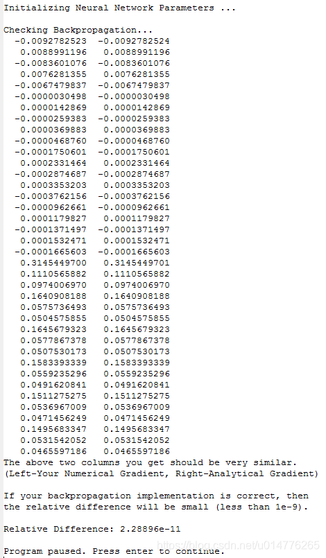
后向传播计算grad梯度与梯度检查：
左边是自己计算的数值梯度，右边是分析梯度（梯度检查的）

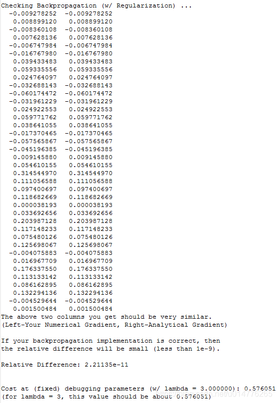
后向传播计算grad梯度与梯度检查加入正则化：
左边是自己计算的数值梯度，右边是分析梯度（梯度检查的）

sigmod梯度值公式：

function g = sigmoidGradient(z)
%SIGMOIDGRADIENT returns the gradient of the sigmoid function
%evaluated at z
%   g = SIGMOIDGRADIENT(z) computes the gradient of the sigmoid function
%   evaluated at z. This should work regardless if z is a matrix or a
%   vector. In particular, if z is a vector or matrix, you should return
%   the gradient for each element.

g = zeros(size(z));

% ====================== YOUR CODE HERE ======================
% Instructions: Compute the gradient of the sigmoid function evaluated at
%               each value of z (z can be a matrix, vector or scalar).

g = sigmoid(z).*(1-sigmoid(z));

% =============================================================

end

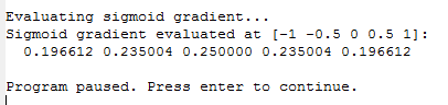
运行结果

sigmod的梯度

ex4.m

%% Machine Learning Online Class - Exercise 4 Neural Network Learning

%  Instructions
%  ------------
% 
%  This file contains code that helps you get started on the
%  linear exercise. You will need to complete the following functions 
%  in this exericse:
%
%     sigmoidGradient.m
%     randInitializeWeights.m
%     nnCostFunction.m
%
%  For this exercise, you will not need to change any code in this file,
%  or any other files other than those mentioned above.
%

%% Initialization
clear ; close all; clc

%% Setup the parameters you will use for this exercise
input_layer_size  = 400;  % 20x20 Input Images of Digits
hidden_layer_size = 25;   % 25 hidden units
num_labels = 10;          % 10 labels, from 1 to 10   
                          % (note that we have mapped "0" to label 10)

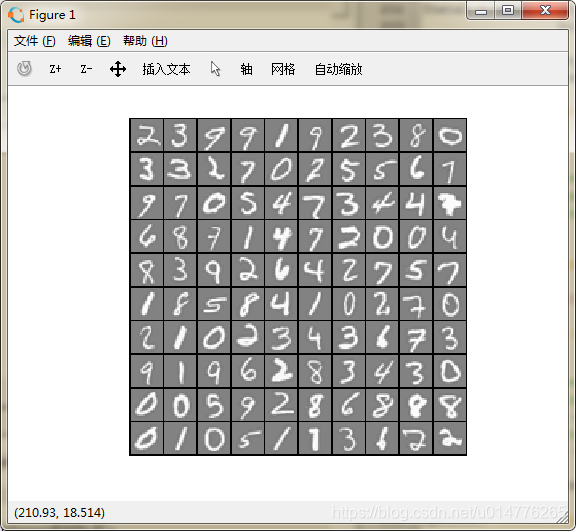
%% =========== Part 1: Loading and Visualizing Data =============
%  We start the exercise by first loading and visualizing the dataset. 
%  You will be working with a dataset that contains handwritten digits.
%

% Load Training Data
fprintf('Loading and Visualizing Data ...\n')

load('ex4data1.mat');
m = size(X, 1);

% Randomly select 100 data points to display
sel = randperm(size(X, 1));
sel = sel(1:100);

displayData(X(sel, :));

fprintf('Program paused. Press enter to continue.\n');
pause;


%% ================ Part 2: Loading Parameters ================
% In this part of the exercise, we load some pre-initialized 
% neural network parameters.

fprintf('\nLoading Saved Neural Network Parameters ...\n')

% Load the weights into variables Theta1 and Theta2
load('ex4weights.mat');

% Unroll parameters 
nn_params = [Theta1(:) ; Theta2(:)];

%% ================ Part 3: Compute Cost (Feedforward) ================
%  To the neural network, you should first start by implementing the
%  feedforward part of the neural network that returns the cost only. You
%  should complete the code in nnCostFunction.m to return cost. After
%  implementing the feedforward to compute the cost, you can verify that
%  your implementation is correct by verifying that you get the same cost
%  as us for the fixed debugging parameters.
%
%  We suggest implementing the feedforward cost *without* regularization
%  first so that it will be easier for you to debug. Later, in part 4, you
%  will get to implement the regularized cost.
%
fprintf('\nFeedforward Using Neural Network ...\n')

% Weight regularization parameter (we set this to 0 here).
lambda = 0;

J = nnCostFunction(nn_params, input_layer_size, hidden_layer_size, ...
                   num_labels, X, y, lambda);

fprintf(['Cost at parameters (loaded from ex4weights): %f '...
         '\n(this value should be about 0.287629)\n'], J);

fprintf('\nProgram paused. Press enter to continue.\n');
pause;

%% =============== Part 4: Implement Regularization ===============
%  Once your cost function implementation is correct, you should now
%  continue to implement the regularization with the cost.
%

fprintf('\nChecking Cost Function (w/ Regularization) ... \n')

% Weight regularization parameter (we set this to 1 here).
lambda = 1;

J = nnCostFunction(nn_params, input_layer_size, hidden_layer_size, ...
                   num_labels, X, y, lambda);

fprintf(['Cost at parameters (loaded from ex4weights): %f '...
         '\n(this value should be about 0.383770)\n'], J);

fprintf('Program paused. Press enter to continue.\n');
pause;


%% ================ Part 5: Sigmoid Gradient  ================
%  Before you start implementing the neural network, you will first
%  implement the gradient for the sigmoid function. You should complete the
%  code in the sigmoidGradient.m file.
%

fprintf('\nEvaluating sigmoid gradient...\n')

g = sigmoidGradient([-1 -0.5 0 0.5 1]);
fprintf('Sigmoid gradient evaluated at [-1 -0.5 0 0.5 1]:\n  ');
fprintf('%f ', g);
fprintf('\n\n');

fprintf('Program paused. Press enter to continue.\n');
pause;


%% ================ Part 6: Initializing Pameters ================
%  In this part of the exercise, you will be starting to implment a two
%  layer neural network that classifies digits. You will start by
%  implementing a function to initialize the weights of the neural network
%  (randInitializeWeights.m)

fprintf('\nInitializing Neural Network Parameters ...\n')

initial_Theta1 = randInitializeWeights(input_layer_size, hidden_layer_size);
initial_Theta2 = randInitializeWeights(hidden_layer_size, num_labels);

% Unroll parameters
initial_nn_params = [initial_Theta1(:) ; initial_Theta2(:)];


%% =============== Part 7: Implement Backpropagation ===============
%  Once your cost matches up with ours, you should proceed to implement the
%  backpropagation algorithm for the neural network. You should add to the
%  code you've written in nnCostFunction.m to return the partial
%  derivatives of the parameters.
%
fprintf('\nChecking Backpropagation... \n');

%  Check gradients by running checkNNGradients
checkNNGradients;

fprintf('\nProgram paused. Press enter to continue.\n');
pause;


%% =============== Part 8: Implement Regularization ===============
%  Once your backpropagation implementation is correct, you should now
%  continue to implement the regularization with the cost and gradient.
%

fprintf('\nChecking Backpropagation (w/ Regularization) ... \n')

%  Check gradients by running checkNNGradients
lambda = 3;
checkNNGradients(lambda);

% Also output the costFunction debugging values
debug_J  = nnCostFunction(nn_params, input_layer_size, ...
                          hidden_layer_size, num_labels, X, y, lambda);

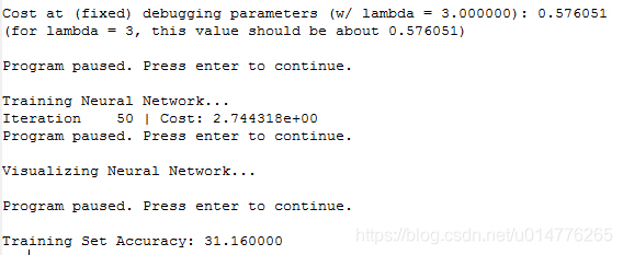
fprintf(['\n\nCost at (fixed) debugging parameters (w/ lambda = %f): %f ' ...
         '\n(for lambda = 3, this value should be about 0.576051)\n\n'], lambda, debug_J);

fprintf('Program paused. Press enter to continue.\n');
pause;


%% =================== Part 8: Training NN ===================
%  You have now implemented all the code necessary to train a neural 
%  network. To train your neural network, we will now use "fmincg", which
%  is a function which works similarly to "fminunc". Recall that these
%  advanced optimizers are able to train our cost functions efficiently as
%  long as we provide them with the gradient computations.
%
fprintf('\nTraining Neural Network... \n')

%  After you have completed the assignment, change the MaxIter to a larger
%  value to see how more training helps.
options = optimset('MaxIter', 50);

%  You should also try different values of lambda
lambda = 1;

% Create "short hand" for the cost function to be minimized
costFunction = @(p) nnCostFunction(p, ...
                                   input_layer_size, ...
                                   hidden_layer_size, ...
                                   num_labels, X, y, lambda);

% Now, costFunction is a function that takes in only one argument (the
% neural network parameters)
[nn_params, cost] = fmincg(costFunction, initial_nn_params, options);

% Obtain Theta1 and Theta2 back from nn_params
Theta1 = reshape(nn_params(1:hidden_layer_size * (input_layer_size + 1)), ...
                 hidden_layer_size, (input_layer_size + 1));

Theta2 = reshape(nn_params((1 + (hidden_layer_size * (input_layer_size + 1))):end), ...
                 num_labels, (hidden_layer_size + 1));

fprintf('Program paused. Press enter to continue.\n');
pause;


%% ================= Part 9: Visualize Weights =================
%  You can now "visualize" what the neural network is learning by 
%  displaying the hidden units to see what features they are capturing in 
%  the data.

fprintf('\nVisualizing Neural Network... \n')

displayData(Theta1(:, 2:end));

fprintf('\nProgram paused. Press enter to continue.\n');
pause;

%% ================= Part 10: Implement Predict =================
%  After training the neural network, we would like to use it to predict
%  the labels. You will now implement the "predict" function to use the
%  neural network to predict the labels of the training set. This lets
%  you compute the training set accuracy.

pred = predict(Theta1, Theta2, X);

fprintf('\nTraining Set Accuracy: %f\n', mean(double(pred == y)) * 100);

运行结果

数据集：

结果：
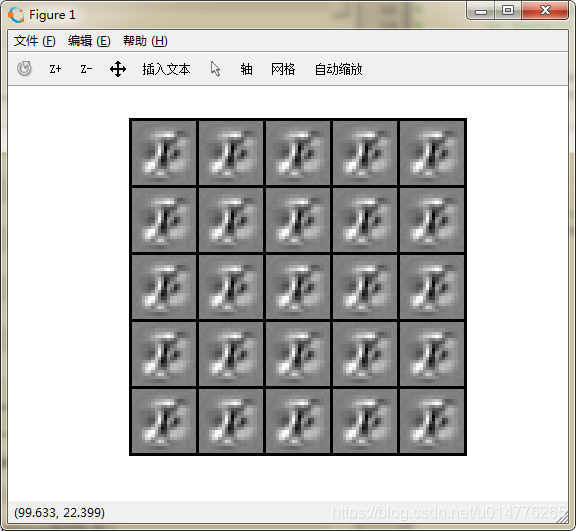
50轮迭代欠拟合，可以看到隐含层中的结果图都一样，且Training Set Accuracy（准确度）仅为31%

修改ex4.m中的MaxIter值

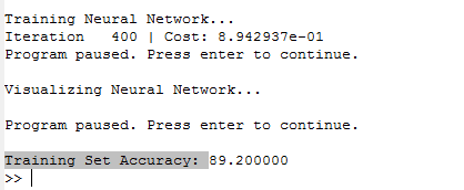
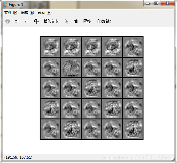
增加迭代轮数，可以看到每一轮迭代cost损失值都在减少，故为正确的。可以看到400轮迭代后，Training Set Accuracy（准确度）提高到89%.可以看到隐含层中的结果图不一样了。

options = optimset('MaxIter', 400);