


注:本文为 “复数” 相关讨论合辑。
英文引文,机翻未校。
如有内容异常,请看原文。
Demystifying complex numbers
揭开复数的神秘面纱
89 At the end of this month I start teaching complex analysis to 2nd year undergraduates, mostly from engineering but some from science and maths. The main applications for them in future studies are contour integrals and Laplace transform, but this should be a “real” complex analysis course which I could later refer to in honours courses. I am now confident (after this discussion, especially Gauss’s complaints given in Keith’s comment) that the name “complex” is discouraging to average students.
89 本月底,我将开始给大二本科生讲授复分析,这些学生大多来自工程专业,也有部分来自理科和数学专业。对他们而言,这门课在未来学习中的主要应用场景是围道积分和拉普拉斯变换,但这应当是一门 “真正的” 复分析课程,方便我后续在荣誉课程中引用。经过此次讨论(尤其是 Keith 的评论中提到的高斯的质疑),我现在确信,“complex”(复杂的)这个名称会让普通学生感到气馁。
Why do we need to study numbers which do not belong to the real world?
我们为何需要学习不属于现实世界的数?
We all know that the thesis is wrong and I have in mind some examples where the use ofcomplexvariable functionssimplifysolving considerably (I give two below). The drawback is that all them assume some knowledge from students already.
我们都清楚这个观点是错误的,而且我想到了一些例子,能说明复变函数的使用可极大简化求解过程(下文给出两个例子)。但缺点是,这些例子都要求学生已具备一定的知识基础。
So I would be happyto learn elementary examples which may convince students that complex numbers and functions of a complex variable are useful.As this question runs in the mode, I would be glad to see one example per answer.
因此,我很乐意了解一些基础例子,帮助学生认识到复数和复变函数的实用性。由于这个问题以该模式推进,我希望每个回答能提供一个例子。
Thank you in advance!
提前感谢大家!
Here are the two promised examples. I was reminded of the second one by several answers and comments about trigonometric functions (and also by the notification that “the bounty on your question Trigonometry related to Rogers–Ramanujan identities expires within three days”; it seems to be harder than I expected).
以下是之前承诺的两个例子。多个关于三角函数的回答和评论让我想到了第二个例子(还有一则通知提到 “关于《罗杰斯 - 拉马努金恒等式相关的三角学》的问题的悬赏将在三天内到期”,这个问题似乎比我预期的更难)。
Example 1. What is the Fourier expansion of the (unbounded) periodic function
例 1:(无界)周期函数的傅里叶展开式是什么?
f ( x ) = ln ∣ sin x 2 ∣ f (x)=\ln\left| \sin \frac {x}{2} \right| f(x)=ln sin2x
*Solution.*The function
f
(
x
)
f (x)
f(x) is periodic with period
2
π
2\pi
2π and has poles at the points
2
π
k
2\pi k
2πk,
k
∈
Z
k \in \mathbb {Z}
k∈Z.
解答:函数
f
(
x
)
f (x)
f(x) 是以
2
π
2\pi
2π 为周期的周期函数,其极点位于
2
π
k
2\pi k
2πk(
k
∈
Z
k \in \mathbb {Z}
k∈Z)处。
Consider the function on the interval
x
∈
[
ε
,
2
π
−
ε
]
x \in [\varepsilon, 2\pi - \varepsilon]
x∈[ε,2π−ε]. The series
考虑该函数在区间
x
∈
[
ε
,
2
π
−
ε
]
x \in [\varepsilon, 2\pi - \varepsilon]
x∈[ε,2π−ε] 上的情况,级数
∑ n = 1 ∞ z n n , z = e i x \sum_{n=1}^{\infty} \frac {z^n}{n}, \quad z=e^{ix} n=1∑∞nzn,z=eix
converges for all values
x
x
x from the interval.
在该区间的所有
x
x
x 值处均收敛。
Since
由于
∣ sin x 2 ∣ = 1 − cos x \left| \sin \frac {x}{2} \right| = \sqrt {1 - \cos x} sin2x =1−cosx
and
Re
ln
w
=
ln
∣
w
∣
\operatorname {Re} \ln w = \ln |w|
Relnw=ln∣w∣, where we choose
w
=
1
2
(
1
−
z
)
w=\frac {1}{2}(1 - z)
w=21(1−z), we deduce that
且
Re
ln
w
=
ln
∣
w
∣
\operatorname {Re} \ln w = \ln |w|
Relnw=ln∣w∣(其中取
w
=
1
2
(
1
−
z
)
w=\frac {1}{2}(1 - z)
w=21(1−z)),由此可推出
Re ( ln 1 − z 2 ) = ln 1 − cos x = ln ∣ sin x 2 ∣ . \operatorname {Re}\left ( \ln \frac {1 - z}{2} \right) = \ln \sqrt {1 - \cos x} = \ln \left| \sin \frac {x}{2} \right|. Re(ln21−z)=ln1−cosx=ln sin2x .
Thus,
因此
ln ∣ sin x 2 ∣ = − ln 2 − Re ∑ n = 1 ∞ z n n = − ln 2 − ∑ n = 1 ∞ cos n x n . \ln \left| \sin \frac {x}{2} \right| = -\ln 2 - \operatorname {Re} \sum_{n=1}^{\infty} \frac {z^n}{n} = -\ln 2 - \sum_{n=1}^{\infty} \frac {\cos nx}{n}. ln sin2x =−ln2−Ren=1∑∞nzn=−ln2−n=1∑∞ncosnx.
As
ε
>
0
\varepsilon > 0
ε>0 can be taken arbitrarily small, the result remains valid for all
x
≠
2
π
k
x \neq 2\pi k
x=2πk.
由于
ε
>
0
\varepsilon > 0
ε>0 可取得任意小,该结果对所有
x
≠
2
π
k
x \neq 2\pi k
x=2πk 均成立。
Example 2. Let
p
p
p be anoddprime number. For an integer
a
a
a relatively prime to
p
p
p, theLegendre symbol
(
a
p
)
\left ( \frac {a}{p} \right)
(pa) is
+
1
+1
+1 or
−
1
-1
−1 depending on whether the congruence
x
2
≡
a
(
m
o
d
p
)
x^2 \equiv a \pmod {p}
x2≡a(modp) is solvable or not. Using the elementary result (a consequence of Fermat’s little theorem) that
例 2:设
p
p
p 为奇素数。对于与
p
p
p 互素的整数
a
a
a,勒让德符号
(
a
p
)
\left ( \frac {a}{p} \right)
(pa) 的取值为
+
1
+1
+1 或
−
1
-1
−1,具体取决于同余式
x
2
≡
a
(
m
o
d
p
)
x^2 \equiv a \pmod {p}
x2≡a(modp) 是否有解。利用(费马小定理的推论这一)基础结论:
( a p ) ≡ a ( p − 1 ) / 2 ( m o d p ) , (*) \left ( \frac {a}{p} \right) \equiv a^{(p-1)/2} \pmod {p}, \tag {*} (pa)≡a(p−1)/2(modp),(*)
show that
证明
( 2 p ) = ( − 1 ) ( p 2 − 1 ) / 8 . \left ( \frac {2}{p} \right) = (-1)^{(p^2 - 1)/8}. (p2)=(−1)(p2−1)/8.
Solution. In the ring
Z
+
Z
i
=
Z
[
i
]
\mathbb {Z} + \mathbb {Z} i = \mathbb {Z}[i]
Z+Zi=Z[i], the binomial formula implies
解答:在环
Z
+
Z
i
=
Z
[
i
]
\mathbb {Z} + \mathbb {Z} i = \mathbb {Z}[i]
Z+Zi=Z[i](高斯整数环)中,由二项式定理可得
( 1 + i ) p ≡ 1 + i p ( m o d p ) . (1 + i)^p \equiv 1 + i^p \pmod {p}. (1+i)p≡1+ip(modp).
On the other hand,
另一方面
( 1 + i ) p = ( 2 e π i / 4 ) p = 2 p / 2 ( cos π p 4 + i sin π p 4 ) (1 + i)^p = \left ( \sqrt {2} e^{\pi i / 4} \right)^p = 2^{p/2} \left ( \cos \frac {\pi p}{4} + i \sin \frac {\pi p}{4} \right) (1+i)p=(2eπi/4)p=2p/2(cos4πp+isin4πp)
and
且
1 + i p = 1 + ( e π i / 2 ) p = 1 + cos π p 2 + i sin π p 2 = 1 + i sin π p 2 . 1 + i^p = 1 + \left ( e^{\pi i / 2} \right)^p = 1 + \cos \frac {\pi p}{2} + i \sin \frac {\pi p}{2} = 1 + i \sin \frac {\pi p}{2}. 1+ip=1+(eπi/2)p=1+cos2πp+isin2πp=1+isin2πp.
Comparing the real parts implies that
比较实部可得
2 p / 2 cos π p 4 ≡ 1 ( m o d p ) , 2^{p/2} \cos \frac {\pi p}{4} \equiv 1 \pmod {p}, 2p/2cos4πp≡1(modp),
hence from
2
cos
(
π
p
/
4
)
∈
{
±
1
}
\sqrt {2} \cos (\pi p / 4) \in \{ \pm 1 \}
2cos(πp/4)∈{±1} we conclude that
因此,由
2
cos
(
π
p
/
4
)
∈
{
±
1
}
\sqrt {2} \cos (\pi p / 4) \in \{ \pm 1 \}
2cos(πp/4)∈{±1} 可推出
2 ( p − 1 ) / 2 ≡ 2 cos π p 4 ( m o d p ) . 2^{(p-1)/2} \equiv \sqrt {2} \cos \frac {\pi p}{4} \pmod {p}. 2(p−1)/2≡2cos4πp(modp).
Then using the elementary result [(*)]:
再利用基础结论 [(*)]:
( 2 p ) ≡ 2 ( p − 1 ) / 2 ≡ 2 cos π p 4 = { 1 if p ≡ ± 1 ( m o d 8 ) , − 1 if p ≡ ± 3 ( m o d 8 ) , \left ( \frac {2}{p} \right) \equiv 2^{(p-1)/2} \equiv \sqrt {2} \cos \frac {\pi p}{4} = \begin {cases} 1 & \text {if } p \equiv \pm 1 \pmod {8}, \\ -1 & \text {if } p \equiv \pm 3 \pmod {8}, \end {cases} (p2)≡2(p−1)/2≡2cos4πp={1−1if p≡±1(mod8),if p≡±3(mod8),
which is exactly the required formula.
这正是所需证明的公式。
edited Jan 4, 2022 at 18:50
Wadim Zudilin
-
Maybe an option is to have them understand that real numbers also do not belong to the real world, that all sort of numbers are simply abstractions.
或许可以让学生理解:实数同样不属于现实世界,所有类型的数都只是抽象概念。
– Mariano Suárez-Álvarez
Commented Jul 1, 2010 at 14:50 -
Probably your electrical engineering students understand better than you do that complex numbers (in polar form) are used to represent amplitude and frequency in their area of study.
你的电气工程专业学生可能比你更清楚:(极坐标形式的)复数在他们的专业领域中用于表示振幅和频率。
– Gerald Edgar
Commented Jul 1, 2010 at 15:36 -
Not an answer, but some suggestions: try reading the beginning of Needham’sVisual Complex Analysis(usf.usfca.edu/vca/) and the end of Levi’s The Mathematical Mechanic(The Mathematical Mechanic: Using Physical Reasoning to Solve Problems).
这并非答案,而是建议:可阅读 Needham 所著《可视化复分析》的开篇,以及 Levi 所著《数学力学:物理推理解决数学问题》的结尾。
– Qiaochu Yuan
Commented Jul 1, 2010 at 17:05 -
Your example has a hidden assumption that a student actually admits the importance of calculating F.S. of ln ∣ sin x 2 ∣ \ln\left| \sin \frac {x}{2} \right| ln sin2x , which I find dubious. The examples with an oscillator’s ODE is more convincing, IMO.
你的例子隐含一个假设:学生认可计算 ln ∣ sin x 2 ∣ \ln\left| \sin \frac {x}{2} \right| ln sin2x 的傅里叶级数(F.S.)的重要性,我对此表示怀疑。在我看来,振动子常微分方程(ODE)相关的例子更具说服力。
– Paul Yuryev
Commented Jul 2, 2010 at 3:02 -
@Mariano, Gerald and Qiaochu: Thanks for the ideas!Visual Complex Analysissounds indeed great, and I’ll follow Levi’s book as soon as I reach the uni library. @Paul: I give the example (which I personally like) and explain that I do not consider it elementary enough for the students. It’s a matter of taste! I’ve never used Fourier series in my own research but it doesn’t imply that I doubt of their importance. We all (including students) have different criteria for measuring such things.
@Mariano、Gerald 和 Qiaochu:感谢这些想法!《Visual Complex Analysis》听起来确实很棒,我一到大学图书馆就会查阅 Levi 的书。@Paul:我给出这个例子(个人很喜欢),并说明它对学生而言不够基础 —— 这是个人偏好问题!我在自己的研究中从未用过傅里叶级数,但这并不意味着我怀疑其重要性,我们所有人(包括学生)对这类事物的衡量标准都不同。
– Wadim Zudilin
Commented Jul 2, 2010 at 5:06
Answers
The nicest elementary illustration I know of the relevance of complex numbers to calculus is its link to radius of convergence, which student learn how to compute by various tests, but more mechanically than conceptually. The series for
1
1
−
x
\frac {1}{1 - x}
1−x1,
log
(
1
+
x
)
\log (1 + x)
log(1+x), and
1
+
x
\sqrt {1 + x}
1+x have radius of convergence 1 and we can see why: there’s a problem at one of the endpoints of the interval of convergence (the function blows up or it’s not differentiable). However, the function
1
1
+
x
2
\frac {1}{1 + x^2}
1+x21 is nice and smooth on the whole real line with no apparent problems, but its radius of convergence at the origin is 1. From the viewpoint of real analysis this is strange: why does the series stop converging? Well, if you look at distance 1 in the complex plane…
我所知道的 “复数与微积分相关性” 的最佳基础例证,是其与收敛半径的关联 —— 学生们会通过各种判别法计算收敛半径,但多是机械操作,而非从概念上理解。级数
1
1
−
x
\frac {1}{1 - x}
1−x1、
log
(
1
+
x
)
\log (1 + x)
log(1+x) 和
1
+
x
\sqrt {1 + x}
1+x 的收敛半径均为 1,原因很明确:收敛区间的某一个端点存在问题(函数趋于无穷或不可微)。但函数
1
1
+
x
2
\frac {1}{1 + x^2}
1+x21 在整个实轴上性质良好且光滑,无明显问题,其在原点处的收敛半径却为 1。从实分析角度看,这很奇怪:级数为何会停止收敛?其实,若在复平面上观察距离为 1 的点……
More generally, you can tell them that for any rational function
p
(
x
)
q
(
x
)
\frac {p (x)}{q (x)}
q(x)p(x), in reduced form, the radius of convergence of this function at a number
a
a
a (on the real line) is precisely the distance from
a
a
a to the nearest zero of the denominator, even if that nearest zero is not real. In other words, to really understand the radius of convergence in a general sense you have to work over the complex numbers. (Yes, there are subtle distinctions between smoothness and analyticity which are relevant here, but you don’t have to discuss that to get across the idea.)
更一般地,可以告诉学生:对于任何既约形式的有理函数
p
(
x
)
q
(
x
)
\frac {p (x)}{q (x)}
q(x)p(x),该函数在(实轴上的)点
a
a
a 处的收敛半径,恰好等于点
a
a
a 到分母最近零点的距离 —— 即便这个最近零点不是实数。换句话说,要从一般意义上真正理解收敛半径,就必须在复数域上研究。(诚然,光滑性与解析性存在细微差别且与此相关,但无需深入讨论即可传达核心思想。)
Similarly, the function
x
e
x
−
1
\frac {x}{e^x - 1}
ex−1x on the real line is smooth, but its power series at
x
=
0
x=0
x=0 has finite radius of convergence
2
π
2\pi
2π (not sure if you can make this numerically apparent). Again, on the real line the reason for this is not visible, but in the complex plane there is a good explanation. If someone is not happy about that function looking initially problematic at
x
=
0
x=0
x=0, where its value is 1, use
x
e
x
+
1
\frac {x}{e^x + 1}
ex+1x instead and the radius of convergence of its power series at
x
=
0
x=0
x=0 has radius of convergence
π
\pi
π rather than
2
π
2\pi
2π.
类似地,实轴上的函数
x
e
x
−
1
\frac {x}{e^x - 1}
ex−1x 性质光滑,但其在
x
=
0
x=0
x=0 处的幂级数收敛半径为有限值
2
π
2\pi
2π(不确定能否通过数值计算直观展示)。同样,在实轴上无法看出缘由,但在复平面上能得到合理解释。若有人觉得该函数在
x
=
0
x=0
x=0 处(函数值为 1)初看有问题,可改用
x
e
x
+
1
\frac {x}{e^x + 1}
ex+1x—— 其在
x
=
0
x=0
x=0 处的幂级数收敛半径为
π
\pi
π,而非
2
π
2\pi
2π。
edited May 4, 2024 at 23:48
2 revs
KConrad
-
Thanks, Keith! That’s a nice point which I always mention for real analysis students as well. The structure of singularities of a linear differential equation (under some mild conditions) fully determines the convergence of the series solving the DE. The generating series for Bernoulli numbers does not produce sufficiently good approximations to 2 π 2\pi 2π, but it’s just beautiful by itself.
谢谢 Keith!这是个很好的观点,我给实分析学生上课时也总会提到。(在一些温和条件下)线性常微分方程(DE)的奇点结构,完全决定了其级数解的收敛性。伯努利数的生成函数虽不能对 2 π 2\pi 2π 给出足够好的逼近,但它本身极具美感。
– Wadim Zudilin
Commented Jul 2, 2010 at 5:14 -
I wouldn’t say itdemystifiesanything.
我不认为这能 “揭开” 任何事物的神秘面纱。
– Incnis Mrsi
Commented Apr 14, 2021 at 4:24 -
@IncnisMrsi my answer was posted almost 11 years ago, so I had to remind myself what the OP’s original request was. It was not about the title, but about the following, taken from the OP’s post: “to learn elementary examples which may convince students in usefulness of complex numbers and functions in complex variable.” Судя по этой просьбе, я думаю, что все в порядке
@IncnisMrsi 我的回答是近 11 年前发布的,所以得回忆提问者(OP)的原始需求。需求与标题无关,而是来自提问者原文:“寻找能让学生相信复数和复变函数有用性的基础例子”。基于这个需求,我认为我的回答是合适的。
– KConrad
Commented Apr 14, 2021 at 5:18 -
My guess is that the main example you cite is the sort of thing that is actually appealing to the already-convinced, i.e. mathematicians who are reading this question, and yet doesn’t necessarily appeal to someone who feels strong and comfortable with some real analysis but doesn’t want to do complex analysis. i.e. it is not at all "strange"from the point of viewof real analysis as to why the series doesn’t converge: The tests that a student has learned for convergence of basic series will show it easily.
我认为你引用的主要例子,实际更能吸引本就认可复数价值的人(即阅读该问题的数学家),但不一定能吸引那些熟悉实分析且得心应手、却不愿学复分析的人。也就是说,从实分析角度看,级数为何不收敛一点也不 “奇怪”—— 学生所学的基础级数收敛判别法就能轻松说明这一点。
– SBK
Commented Jun 11, 2024 at 14:41 -
@SBK I of course am already convinced, but I still think an appropriately thoughtful student might wonderwhythe real analysis convergence tests are saying the radius of convergence is a value R R R when nothing appears to be going wrong at x = ± R x=\pm R x=±R (a contrast to the series for 1 1 − x \frac {1}{1 - x} 1−x1 and log ( 1 + x ) \log (1 + x) log(1+x) at x = 0 x=0 x=0, where R = 1 R=1 R=1).
@SBK 我当然本就认可复数的价值,但仍认为善于思考的学生可能会疑惑:为何实分析收敛判别法得出收敛半径为 R R R,而在 x = ± R x=\pm R x=±R 处却看似无问题(这与 1 1 − x \frac {1}{1 - x} 1−x1 和 log ( 1 + x ) \log (1 + x) log(1+x) 在 x = 0 x=0 x=0 处的级数形成对比 —— 后者收敛半径 R = 1 R=1 R=1,且端点处存在问题)。
– KConrad
Commented Jun 11, 2024 at 23:57
You can solve the differential equation
y
′
′
+
y
=
0
y'' + y = 0
y′′+y=0 using complex numbers. Just write
可利用复数求解微分方程
y
′
′
+
y
=
0
y'' + y = 0
y′′+y=0,只需写成
( ∂ 2 + 1 ) y = ( ∂ + i ) ( ∂ − i ) y (\partial^2 + 1) y = (\partial + i)(\partial - i) y (∂2+1)y=(∂+i)(∂−i)y
and you are now dealing with two order one differential equations that are easily solved
这样就转化为两个易于求解的一阶微分方程:
( ∂ + i ) z = 0 , ( ∂ − i ) y = z . (\partial + i) z = 0, \quad (\partial - i) y = z. (∂+i)z=0,(∂−i)y=z.
The multivariate case is a bit harder and uses quaternions or Clifford algebras. This was done by Dirac for the Schrodinger equation
−
Δ
ψ
=
i
∂
t
ψ
-\Delta \psi = i \partial_t \psi
−Δψ=i∂tψ, and that led him to the prediction of the existence of antiparticles (and to the Nobel prize).
多变量情况稍复杂,需用到四元数或克利福德代数。狄拉克(Dirac)曾将此方法用于薛定谔方程
−
Δ
ψ
=
i
∂
t
ψ
-\Delta \psi = i \partial_t \psi
−Δψ=i∂tψ,进而预言了反粒子的存在(并因此获诺贝尔奖)。
edited May 5, 2024 at 4:33
coudy
-
Thanks, coudy! This is really nice (Pietro’s answer only hints a possible use of 2nd order DEs).
谢谢 coudy!这个例子非常好(Pietro 的回答仅暗示了二阶常微分方程(DEs)的一种可能用途)。
– Wadim Zudilin
Commented Jul 1, 2010 at 12:24 -
I was taught a similar trick as a second-year honours undergraduate (same target that the OP suggests), and I don’t find it helpful at all. The problem is that you’ll probably need to spend a full lecture trying to formalize it and explain why it works, otherwise it just looks like a magical unmotivated trick that abuses notation.
我在大二荣誉课程(与提问者提到的目标学生群体相同)中也学过类似方法,但认为它毫无帮助。问题在于:你可能需要一整节课来将其形式化并解释原理,否则它看起来就像无依据的 “魔法技巧”,还滥用了符号。
– Federico Poloni
Commented Jan 27, 2014 at 11:30 -
@Frederico: why do you say it abuses notation? That would be true in higher dimensional case without introducing Clifford algebras. But here it’s perfectly valid. You just need to know what complex numbers are.
@Frederico:你为何说它滥用符号?在不引入克利福德代数的高维情况下确实如此,但这个例子中完全有效 —— 你只需理解复数是什么即可。
– Marek
Commented Jan 27, 2014 at 15:09 -
How is Dirac theory based on (parabolic) Schrödinger equation? We know that a solution to Dirac equation is a solution to Klein–Gordon equation which is hyperbolic.
狄拉克理论如何基于(抛物型的)薛定谔方程?我们知道,狄拉克方程的解是双曲型克莱因 - 戈登方程的解。
– Incnis Mrsi
Commented Apr 14, 2021 at 4:29 -
@Marek I see only now this old comment but I’ll answer anyway just in case. The ‘abuse of notation’ is that it at that point students do not know that ∂ \partial ∂ belongs to an operator algebra and that it makes sense to factor out ∂ 2 y + y = ( ∂ 2 + 1 ) y \partial^2 y + y = (\partial^2 + 1) y ∂2y+y=(∂2+1)y, let alone decompose it as ( ∂ + i ) ( ∂ − i ) (\partial + i)(\partial - i) (∂+i)(∂−i). The fact that the derivative notation ∂ 2 y \partial^2 y ∂2y reads like a square followed by a product by y y y at that point is just notation, so this seems to belong to the same category as simplifying out d x dx dx to change variables in integrals.
@Marek 我现在才看到这条旧评论,但还是回复一下以防有人需要。所谓 “滥用符号”,是因为这个阶段的学生不知道 ∂ \partial ∂ 属于算子代数,也不理解将 ∂ 2 y + y = ( ∂ 2 + 1 ) y \partial^2 y + y = (\partial^2 + 1) y ∂2y+y=(∂2+1)y 因式分解的合理性,更不用说分解为 ( ∂ + i ) ( ∂ − i ) (\partial + i)(\partial - i) (∂+i)(∂−i) 了。此时,导数符号 ∂ 2 y \partial^2 y ∂2y 看起来像 “先平方再乘以 y y y”,这本质上只是符号表示,因此这种做法与积分变量替换中消去 d x dx dx 类似,都属于符号滥用。
– Federico Poloni
Commented Apr 14, 2021 at 6:43
Students usually find the connection of trigonometric identities like
sin
(
a
+
b
)
=
sin
a
cos
b
+
cos
a
sin
b
\sin (a + b) = \sin a \cos b + \cos a \sin b
sin(a+b)=sinacosb+cosasinb to multiplication of complex numbers striking.
学生通常会觉得三角恒等式如
sin
(
a
+
b
)
=
sin
a
cos
b
+
cos
a
sin
b
\sin (a + b) = \sin a \cos b + \cos a \sin b
sin(a+b)=sinacosb+cosasinb 与复数乘法之间的联系令人惊讶。
edited Jul 1, 2010 at 14:12
Not sure about the students, but I do.
我不确定学生们是否如此,但我确实如此。
– Wadim Zudilin
Commented Jul 1, 2010 at 12:21
Well, I am not claiming this about all students, but whenever I mentioned this (or same things in terms of rotation matrices) in class, I always get excited feedback at least from some of them.
嗯,我不是说所有学生都这样,但每当我提到这个(或者在旋转矩阵方面提到类似的内容)时,我总是会从至少一些学生那里得到积极的反馈。
– Yuri Bakhtin
Commented Jul 1, 2010 at 12:24
This is an excellent suggestion. I can never remember these identities off the top of my head. Whenever I need one of them, the simplest way (faster than googling) is to read them off from
(
a
+
i
b
)
(
c
+
i
d
)
=
(
a
c
−
b
d
)
+
i
(
a
d
+
b
c
)
(a + ib)(c + id) = (ac - bd) + i (ad + bc)
(a+ib)(c+id)=(ac−bd)+i(ad+bc).
这是一个很好的建议。我永远记不住这些恒等式。每当我需要其中一个时,最简单的方法(比谷歌搜索还快)就是从
(
a
+
i
b
)
(
c
+
i
d
)
=
(
a
c
−
b
d
)
+
i
(
a
d
+
b
c
)
(a + ib)(c + id) = (ac - bd) + i (ad + bc)
(a+ib)(c+id)=(ac−bd)+i(ad+bc) 中读取它们。
– alex
Commented Jul 1, 2010 at 20:35
When I first started teaching calculus in the US, I was surprised that many students didn’t remember addition formulas for trig functions. As the years went by, it’s gotten worse: now the whole idea of using an identity like that to solve a problem is alien to them, e.g. even if they may look it up doing the homework, they “get stuck” on the problem and “don’t get it”. What is there to blame: calculators? standard tests that neglect it? teachers who never understood it themselves? Anyway, it’s a very bad omen.
当我刚开始在美国教微积分时,我很惊讶许多学生不记得三角函数的加法公式。随着时间的推移,情况变得更糟:现在,使用这样的恒等式来解决问题的想法对他们来说是陌生的,例如,即使他们在做作业时可能会查找它,他们也会在问题上 “卡住” 并且 “不明白”。该责怪什么呢:计算器?忽视这一点的标准测试?还是那些自己从未理解它的老师?不管怎样,这是一个非常不好的兆头。
– Victor Protsak
Commented Jul 2, 2010 at 1:43
@Victor: It can be worse… When I taught Calc I at U of Toronto to engineering students, I was approached by some students who claimed they had heard words “sine” and “cosine” but were not quite sure what they meant.
@Victor:情况可能会更糟…… 当我给多伦多大学的工程系学生教授微积分 I 时,一些学生找到我,声称他们听说过 “正弦” 和 “余弦” 这些词,但不太确定它们的含义。
– Yuri Bakhtin
Commented Jul 2, 2010 at 8:51
From “Birds and Frogs” by Freeman Dyson [Notices of Amer. Math. Soc. 56 (2009) 212–223]:
来自弗里曼・戴森的《鸟与蛙》[Notices of Amer. Math. Soc. 56 (2009) 212–223]:
One of the most profound jokes of nature is the square root of minus one that the physicist Erwin Schrödinger put into his wave equation when he invented wave mechanics in 1926. Schrödinger was a bird who started from the idea of unifying mechanics with optics. A hundred years earlier, Hamilton had unified classical mechanics with ray optics, using the same mathematics to describe optical rays and classical particle trajectories. Schrödinger’s idea was to extend this unification to wave optics and wave mechanics. Wave optics already existed, but wave mechanics did not. Schrödinger had to invent wave mechanics to complete the unification. Starting from wave optics as a model, he wrote down a differential equation for a mechanical particle, but the equation made no sense. The equation looked like the equation of conduction of heat in a continuous medium. Heat conduction has no visible relevance to particle mechanics. Schrödinger’s idea seemed to be going nowhere. But then came the surprise. Schrödinger put the square root of minus one into the equation, and suddenly it made sense. Suddenly it became a wave equation instead of a heat conduction equation. And Schrödinger found to his delight that the equation has solutions corresponding to the quantized orbits in the Bohr model of the atom. It turns out that the Schrödinger equation describes correctly everything we know about the behavior of atoms. It is the basis of all of chemistry and most of physics. And that square root of minus one means that nature works with complex numbers and not with real numbers. This discovery came as a complete surprise, to Schrödinger as well as to everybody else. According to Schrödinger, his fourteen-year-old girl friend Itha Junger said to him at the time, “Hey, you never even thought when you began that so much sensible stuff would come out of it.” All through the nineteenth century, mathematicians from Abel to Riemann and Weierstrass had been creating a magnificent theory of functions of complex variables. They had discovered that the theory of functions became far deeper and more powerful when it was extended from real to complex numbers. But they always thought of complex numbers as an artificial construction, invented by human mathematicians as a useful and elegant abstraction from real life. It never entered their heads that this artificial number system that they had invented was in fact the ground on which atoms move. They never imagined that nature had got there first.
自然界最深刻的玩笑之一是物理学家埃尔温・薛定谔在 1926 年发明波动力学时将负一的平方根放入他的波动方程中。薛定谔是一个从统一力学和光学的想法出发的 “鸟”。一百年前,哈密顿已经用相同的数学描述光学射线和经典粒子轨迹,统一了经典力学和射线光学。薛定谔的想法是将这种统一扩展到波动光学和波动力学。波动光学已经存在,但波动力学还没有。薛定谔必须发明波动力学以完成这种统一。以波动光学为模型,他为一个机械粒子写下了一个微分方程,但这个方程毫无意义。这个方程看起来像是连续介质中热传导的方程。热传导与粒子力学没有明显的关联。薛定谔的想法似乎走到了死胡同。但随后出现了惊喜。薛定谔在方程中加入了负一的平方根,突然间它变得有意义了。它突然变成了一个波动方程,而不是热传导方程。薛定谔高兴地发现,这个方程的解对应于玻尔原子模型中的量子轨道。事实证明,薛定谔方程正确地描述了我们所知道的原子的一切行为。它是所有化学和大部分物理学的基础。而那个负一的平方根意味着自然界使用复数而不是实数。这一发现对薛定谔以及其他人来说都是一个完全的惊喜。据薛定谔说,他当时 14 岁的女朋友伊塔・容格对他说:“嘿,你一开始甚至没想到会有这么多合理的东西从中产生。” 在整个 19 世纪,从阿贝尔到黎曼和魏尔斯特拉斯的数学家们一直在创造一个关于复变量函数的宏伟理论。他们发现,当函数理论从实数扩展到复数时,它变得更加深刻和强大。但他们总是把复数当作一个由人类数学家发明的有用且优雅的现实生活的抽象构造。他们从未想过他们发明的这种人造数系实际上是原子运动的基础。他们从未想过大自然已经先一步到达那里。
answered Jul 9, 2010 at 12:12
– Wadim Zudilin
As discussed at physics.stackexchange.com/questions/428033/… putting in an imaginary diffusion coefficient into the heat equation changes the equation to become invariant against time reversal
t
→
−
t
t \to -t
t→−t like a wave equation. This is what Dyson means with “it suddenly made sense”.
正如在 physics.stackexchange.com/questions/428033/… 中讨论的那样,将一个虚数扩散系数放入热方程中会使方程变得像波动方程一样对时间反演
t
→
−
t
t \to -t
t→−t 不变。这就是戴森所说的 “它突然变得有意义了”。
– user4503
Commented Oct 7, 2018 at 19:57
If the students have had a first course in differential equations, tell them to solve the system
如果学生们已经上过微分方程的入门课程,让他们解这个方程组:
x
′
(
t
)
=
−
y
(
t
)
x'(t) = -y (t)
x′(t)=−y(t)
y
′
(
t
)
=
x
(
t
)
y'(t) = x (t)
y′(t)=x(t).
This is the equation of motion for a particle whose velocity vector is always perpendicular to its displacement. Explain why this is the same thing as
这是速度向量始终与其位移垂直的粒子的运动方程。解释为什么这与
( x ( t ) + i y ( t ) ) ′ = i ( x ( t ) + i y ( t ) ) (x (t) + iy (t))' = i (x (t) + iy (t)) (x(t)+iy(t))′=i(x(t)+iy(t))
hence that, with the right initial conditions, the solution is
是一样的,因此在适当的初始条件下,解为
x ( t ) + i y ( t ) = e i t x (t) + iy (t) = e^{it} x(t)+iy(t)=eit.
On the other hand, a particle whose velocity vector is always perpendicular to its displacement travels in a circle. Hence, again with the right initial conditions, x(t)=cost,y(t)=sint (At this point you might reiterate that complex numbers are real 2×2 matrices, assuming they have seen this method for solving systems of differential equations.)
另一方面,速度向量始终与其位移垂直的粒子沿圆周运动。因此,同样在适当的初始条件下,
x
(
t
)
=
cos
t
x (t) = \cos t
x(t)=cost,
y
(
t
)
=
sin
t
y (t) = \sin t
y(t)=sint(此时你可能会重申复数是实数 2×2 矩阵,假设他们已经见过这种解微分方程组的方法。)
answered Jul 1, 2010 at 17:11
– Qiaochu Yuan
Thanks, Qiaochu! They have some background in DEs, and this is a very good way to get DEs, trig identities and matrices at the same time.
谢谢,Qiaochu!他们有一些微分方程的背景,这是一个同时涉及微分方程、三角恒等式和矩阵的非常好的方法。
– Wadim Zudilin
Commented Jul 2, 2010 at 5:43
I just used basically this in a first course in differential equations to prove Euler’s formula for them. One of us thought it was really cool, anyway…
我刚刚在微分方程的入门课程中用这个来证明欧拉公式。我们中有人觉得这真的很酷……
– Ryan Reich
Commented Mar 22, 2013 at 14:10
Here are two simple uses of complex numbers that I use to try to convince students that complex numbers are “cool” and worth learning.
这里有两种简单的复数用法,我用它们来说服学生复数是 “酷” 的,值得学习。
-
(Number Theory) Use complex numbers to derive Brahmagupta’s identity expressing ( a 2 + b 2 ) ( c 2 + d 2 ) (a^2 + b^2)(c^2 + d^2) (a2+b2)(c2+d2) as the sum of two squares, for integers a,b,c,d.
(数论)利用复数推导婆罗摩笈多恒等式,将 ( a 2 + b 2 ) ( c 2 + d 2 ) (a^2 + b^2)(c^2 + d^2) (a2+b2)(c2+d2) 表示为两个平方数之和,其中 a,b,c,d 是整数。 -
(Euclidean geometry) Use complex numbers to explain Ptolemy’s Theorem. For a cyclic quadrilateral with vertices A,B,C,D we have
(欧几里得几何)利用复数解释托勒密定理。对于一个圆内接四边形,其顶点为 A,B,C,D,我们有
A C ‾ ⋅ B D ‾ = A B ‾ ⋅ C D ‾ + B C ‾ ⋅ A D ‾ \overline {AC} \cdot \overline {BD} = \overline {AB} \cdot \overline {CD} + \overline {BC} \cdot \overline {AD} AC⋅BD=AB⋅CD+BC⋅AD.
edited Jul 1, 2010 at 16:15
And even more amazingly, one can completely solve the diophantine equation
x
2
+
y
2
=
z
n
x^2 + y^2 = z^n
x2+y2=zn for any n as follows:
更令人惊讶的是,我们可以完全解决任何 n 的丢番图方程
x
2
+
y
2
=
z
n
x^2 + y^2 = z^n
x2+y2=zn,如下:
x + y i = ( a + b i ) n x + yi = (a + bi)^n x+yi=(a+bi)n, z = a 2 + b 2 z = a^2 + b^2 z=a2+b2.
I learned this from a popular math book while in elementary school, many years before studying calculus.
我在小学时从一本通俗数学书中了解到这一点,这比学习微积分早了很多年。
– Victor Protsak
Commented Jul 2, 2010 at 1:21
@Byron: Thanks! 2 examples in one answer: I can vote only once.
@Victor: I am indeed amazed! This elementary knowledge is new to me. I probably spent too much on complex DEs…
@Byron:谢谢!一个回答中有两个例子:我只能投一次票。
@Victor:我确实很惊讶!这些基本知识对我来说是新的。我可能在复微分方程上花的时间太多了……
– Wadim Zudilin
Commented Jul 2, 2010 at 5:21
How does the vector calculus identity explain complex numbers? It is about an inner product space, true in every dimension (and not necessary for a positive-definite scalar product). There is dot product in every
R
n
R^n
Rn,n≥1 , but only for n=1,2,4 multiplication exists (and only for n=1,2 is it commutative). Downvote.
向量微积分恒等式如何解释复数?它涉及内积空间,适用于所有维度(并且不需要正定标量积)。在每个
R
n
R^n
Rn,n≥1 中都有点积,但只有在 n=1,2,4 时才存在乘法(并且只有在 n=1,2 时它是可交换的)。反对。
– Incnis Mrsi
Commented Apr 14, 2021 at 4:49
One cannot over - emphasize that passing to complex numbers often permits a great simplification by linearizing what would otherwise be more complex nonlinear phenomena. One example familiar to any calculus student is the fact that integration of rational functions is much simpler over
C
\mathbb {C}
C (vs.
R
\mathbb {R}
R) since partial fraction decompositions involve at most linear (vs quadratic) polynomials in the denominator. Similarly one reduces higher - order constant coefficient differential and difference equations to linear (first - order) equations by factoring the linear operators over
C
\mathbb {C}
C. More generally one might argue that such simplification by linearization was at the heart of the development of abstract algebra. Namely, Dedekind, by abstracting out the essential linear structures (ideals and modules) in number theory, greatly simplified the prior nonlinear theory based on quadratic forms. This enabled him to exploit to the hilt the power of linear algebra. Examples abound of the revolutionary power that this brought to number theory and algebra - e.g. for one little - known gem see my recent post explaining how Dedekind’s notion of conductor ideal beautifully encapsulates the essence of elementary irrationality proofs of n’th roots.
不能过分强调,转向复数常常可以通过 “线性化” 来极大地简化那些否则会更复杂的 “非线性” 现象。每一个微积分学生都熟悉的例子是,由于部分分式分解在分母中最多只涉及一次(而不是二次)多项式,有理函数在
C
\mathbb {C}
C 上的积分(与在
R
\mathbb {R}
R 上相比)要简单得多。同样,通过在
C
\mathbb {C}
C 上分解线性算子,人们可以把高阶常系数微分方程和差分方程简化为线性(一阶)方程。更一般地说,有人可能会认为,这种 “通过线性化来简化” 是抽象代数发展的核心。具体来说,戴德金通过抽象出数论中的基本线性结构(理想和模),极大地简化了此前基于二次型的非线性理论。这使他能够充分利用线性代数的力量。这种变革性的力量在数论和代数中带来了无数的例子,例如,我最近的一篇文章解释了戴德金的 “导子理想” 概念如何优美地概括了 n 次根初等无理性证明的本质,这是一颗鲜为人知的明珠。
edited Jun 15, 2020 at 7:27
– Bill Dubuque
If you really want to “demystify” complex numbers, I’d suggest teaching what complex multiplication looks like with the following picture, as opposed to a matrix representation:
如果你真想 “揭开复数的神秘面纱”,我建议用下面的形象化,而不是矩阵表示法,来教复数乘法是什么样的:
If you want to visualize the product “z w”, start with ‘0’ and ‘w’ in the complex plane, then make a new complex plane where ‘0’ sits above ‘0’ and ‘1’ sits above ‘w’. If you look for ‘z’ up above, you see that ‘z’ sits above something you name ‘z w’. You could teach this picture for just the real numbers or integers first – the idea of using the rest of the points of the plane to do the same thing is a natural extension.
如果你想形象化 “z w” 这个乘积,先在复平面上找到 “0” 和 “w”,然后做一个新的复平面,让 “0” 在 “0” 的上方,“1” 在 “w” 的上方。如果你在上方找 “z”,你会看到 “z” 在你命名为 “z w” 的东西的上方。你可以先用这个图形来教实数或整数的乘法 —— 用平面上的其他点来做同样的事是很自然的扩展。
You can use this picture to visually “demystify” a lot of things:
你可以用这个图形来形象地 “揭开” 很多事情的 “神秘面纱”:
-
Why is a negative times a negative a positive? — I know some people who lost hope in understanding math as soon as they were told this fact.
为什么负数乘以负数等于正数?—— 我知道有些人一听到这个事实就对理解数学失去了信心。 -
i 2 = − 1 i^2 = -1 i2=−1
-
( z w ) t = z ( w t ) \left (zw\right) t = z\left (wt\right) (zw)t=z(wt) — I think this is a better explanation than a matrix representation as to why the product is associative.
( z w ) t = z ( w t ) \left (zw\right) t = z\left (wt\right) (zw)t=z(wt)—— 我认为这比矩阵表示法更能解释为什么乘法是结合的。∣ z w ∣ = ∣ z ∣ ∣ w ∣ \lvert zw \rvert = \lvert z \rvert \lvert w \rvert ∣zw∣=∣z∣∣w∣
( z + w ) v = z v + w v \left (z + w\right) v = zv + wv (z+w)v=zv+wv -
The Pythagorean Theorem: draw ( 1 − i t ) ( 1 + i t ) = 1 + t 2 \left (1 - it\right)\left (1 + it\right) = 1 + t^2 (1−it)(1+it)=1+t2 etc.
勾股定理:画出 ( 1 − i t ) ( 1 + i t ) = 1 + t 2 \left (1 - it\right)\left (1 + it\right) = 1 + t^2 (1−it)(1+it)=1+t2 等等。
One thing that’s not so easy to see this way is the commutativity (for good reasons).
用这种方式不太容易看出交换性(这是有原因的)。
After everyone has a grasp on how complex multiplication looks, you can get into the differential equation: d z d t = i z \frac {dz}{dt} = iz dtdz=iz, z ( 0 ) = 1 z\left (0\right) = 1 z(0)=1 which Qiaochu noted travels counterclockwise in a unit circle at unit speed. You can use it to give a good definition for sine and cosine – in particular, you get to define π \pi π as the smallest positive solution to e i π = − 1 e^{i\pi} = -1 eiπ=−1. It’s then physically obvious (as long as you understand the multiplication) that e i ( x + y ) = e i x e i y e^{i\left (x + y\right)} = e^{ix} e^{iy} ei(x+y)=eixeiy, and your students get to actually understand all those hard/impossible to remember facts about trig functions (like angle addition and derivatives) that they were forced to memorize earlier in their lives. It may also be fun to discuss how the picture for ( 1 + z n ) n \left (1 + \frac {z}{n}\right)^n (1+nz)n turns into a picture of that differential equation in the “compound interest” limit as n → ∞ n \to \infty n→∞; doing so provides a bridge to power series, and gives an opportunity to understand the basic properties of the real exponential function more intuitively as well.
在每个人都知道复数乘法是什么样子之后,你可以进入微分方程 d z d t = i z \frac {dz}{dt} = iz dtdz=iz, z ( 0 ) = 1 z\left (0\right) = 1 z(0)=1,Qiaochu 指出它以单位速度在单位圆中逆时针运动。你可以用它来很好地定义正弦和余弦 —— 特别是,你可以将 π \pi π 定义为 e i π = − 1 e^{i\pi} = -1 eiπ=−1 的最小正解。只要理解了乘法, e i ( x + y ) = e i x e i y e^{i\left (x + y\right)} = e^{ix} e^{iy} ei(x+y)=eixeiy 就是显而易见的,你的学生们实际上可以理解那些他们以前被迫记住的关于三角函数的难以 / 不可能记住的事实(比如角度加法和导数)。讨论 ( 1 + z n ) n \left (1 + \frac {z}{n}\right)^n (1+nz)n 的图形如何在 n → ∞ n \to \infty n→∞ 的 “复利” 极限中变成那个微分方程的图形也许会很有趣;这样做提供了一个通往幂级数的桥梁,并且也提供了一个机会,让人们更直观地理解实指数函数的基本性质。
But this stuff is less demystifying complex numbers and more… demystifying other stuff using complex numbers.
但这些东西较少地是揭开复数的神秘面纱,而更多地是…… 用复数来揭开其他东西的神秘面纱。
Here’s a link to some Feynman lectures on Quantum Electrodynamics (somehow prepared for a general audience) if you really need some flat out real - world complex numbers
如果你真的需要一些纯正的现实世界中的复数,这里有一些费曼关于量子电动力学的演讲的链接(不知何故是为普通观众准备的)
http://video.google.com.au/videosearch?q=feynman+auckland&filter=0&start=0#
answered Jul 2, 2010 at 2:50
– Phil Isett
One of my favourite elementary applications of complex analysis is the evaluation of infinite sums of the form
我最喜欢的复分析初等应用之一是利用留数来计算如下形式的无穷级数
∑ n ≥ 0 p ( n ) q ( n ) \sum\limits_{n \geq 0} \frac {p (n)}{q (n)} n≥0∑q(n)p(n)
where p,q are polynomials and deg q>1+degp , by using residues.
其中 p,q 是多项式,且
deg
q
>
1
+
deg
p
\deg q > 1 + \deg p
degq>1+degp。
answered Jul 1, 2010 at 9:25
– José Figueroa - O’Farrill
Thanks, José! This was not my list (even I use this very often in serious problems). I only wonder whether it is possible to start a course with such example.
谢谢,José!这不是我的列表(即使我在严肃的问题中经常使用它)。我只是想知道是否可以用这样的例子开始一门课程。
– Wadim Zudilin
Commented Jul 1, 2010 at 10:01
They’re useful just for doing ordinary geometry when programming.
它们在编程时用于普通的几何运算也很有用。
A common pattern I have seen in a great many computer programs is to start with a bunch of numbers that are really ratios of distances. These numbers get converted to angles with inverse trig functions. Then some simple functions are applied to the angles and the trig functions are used on the results.
我在许多计算机程序中常见的一种模式是,先从一堆实际上是距离比的数字开始。这些数字通过反三角函数转换为角度。然后对这些角度应用一些简单的函数,并对结果使用三角函数。
Trig and inverse trig functions are expensive to compute on a computer. In high - performance code you want to eliminate them if possible. Quite often, for the above case, you can eliminate the trig functions. For example
cos
(
2
cos
−
1
x
)
=
2
x
2
−
1
\cos (2\cos^{-1} x) = 2x^2 - 1
cos(2cos−1x)=2x2−1( (for
x
x
x in a suitable range) but the version on the right runs much faster.
在计算机上计算三角函数和反三角函数是很费时的。在高性能代码中,如果可能的话,你希望消除它们。在上述情况下,你常常可以消除三角函数。例如,
cos
(
2
cos
−
1
x
)
=
2
x
2
−
1
\cos (2\cos^{-1} x) = 2x^2 - 1
cos(2cos−1x)=2x2−1(对于合适的范围内的 x),但右边的版本运行速度要快得多。
The catch is remembering all those trig formulae. It’d be nice to make the compiler do all the work. A solution is to use complex numbers. Instead of storing θ we store (cosθ,sinθ) . We can add angles by using complex multiplication, multiply angles by integers and rational numbers using powers and roots and so on. As long as you don’t actually need the numerical value of the angle in radians you need never use trig functions. Obviously there comes a point where the work of doing operations on complex numbers may outweigh the saving of avoiding trig. But often in real code the complex number route is faster.
问题是记住所有这些三角公式。最好能让编译器来做所有这些工作。一个解决办法是使用复数。我们不是存储 θ,而是存储 (cosθ,sinθ)。我们可以通过复数乘法来加角度,通过使用幂和根等来用整数和有理数乘角度。只要实际上不需要角度的弧度数值,就永远不需要使用三角函数。显然,到了一定时候,对复数进行运算的工作量可能会超过避免使用三角函数所节省下来的量。但在实际代码中,常常走复数这条路更快。
(Of course it’s analogous to using quaternions for rotations in 3D. I guess it’s somewhat in the spirit of rational trigonometry except I think it’s easier to work with complex numbers.)
(当然,这与在三维中用四元数进行旋转是类似的。我想这有点类似于 有理三角学 的精神,不过我认为使用复数更容易。)
answered Jul 2, 2010 at 4:23
– Dan Piponi
Thanks! Your answer and Victor’s comments reminded me about a related deduction in number theory (I’ll try to add one more example to the original question).
谢谢!你的回答和 Victor 的评论让我想起了数论中的一个相关推论(我会试着在原问题中再加一个例子)。
– Wadim Zudilin
Commented Jul 2, 2010 at 8:46
This answer is an expansion of the answer of Yuri Bakhtin.
这个回答是对尤里・巴赫京的回答的扩展。
Here is a kind of mime show.
这是一个哑剧表演。
Silently write the formulas for
cos
(
2
x
)
\cos (2x)
cos(2x) and
sin
(
2
x
)
\sin (2x)
sin(2x) lined up on the board, something like this:
在黑板上默默地写下
cos
(
2
x
)
\cos (2x)
cos(2x) 和
sin
(
2
x
)
\sin (2x)
sin(2x) 的公式,像这样排列:
cos ( 2 x ) = cos 2 ( x ) − sin 2 ( x ) sin ( 2 x ) = + 2 cos ( x ) sin ( x ) \cos (2x) = \cos^2 (x) - \sin^2 (x) \\ \sin (2x) = +2\cos (x)\sin (x) cos(2x)=cos2(x)−sin2(x)sin(2x)=+2cos(x)sin(x)
Do the same for the formulas for cos ( 3 x ) \cos (3x) cos(3x) and sin ( 3 x ) \sin (3x) sin(3x), and however far you want to go:
对 cos ( 3 x ) \cos (3x) cos(3x) 和 sin ( 3 x ) \sin (3x) sin(3x) 的公式也做同样的事情,你想写多远就写多远:
cos ( 3 x ) = cos 3 ( x ) − 3 cos ( x ) sin 2 ( x ) sin ( 3 x ) = + 3 cos 2 ( x ) sin ( x ) − sin 3 ( x ) \cos (3x) = \cos^3 (x) - 3\cos (x)\sin^2 (x) \\ \sin (3x) = +3\cos^2 (x)\sin (x) - \sin^3 (x) cos(3x)=cos3(x)−3cos(x)sin2(x)sin(3x)=+3cos2(x)sin(x)−sin3(x)
Maybe then let out a loud noise like “hmmmmmmmmm… I recognize those numbers…”
然后也许发出一声像 “hmmmmmmmmm… 我认得那些数字……” 这样的大声嘟囔。
Then, on a parallel board, write out Pascal’s triangle, and parallel to that write the application of Pascal’s triangle to the binomial expansions
(
x
+
y
)
n
(x + y)^n
(x+y)n. Make some more puzzling sounds regarding those pesky plus and minus signs.
然后,在一个平行的黑板上,写出帕斯卡三角形,并且在它旁边写出杨辉三角形在二项式展开式
(
x
+
y
)
n
(x + y)^n
(x+y)n 中的应用。再对那些讨厌的正负号发出一些困惑的声音。
Then maybe it’s time to actually say something: “Eureka! We can tie this all together by use of an imaginary number
i
=
−
1
i = \sqrt {-1}
i=−1.” Then write out the binomial expansion of
然后也许到了该说些什么的时候了:“尤里卡!我们可以通过使用虚数
i
=
−
1
i = \sqrt {-1}
i=−1 把这一切联系起来。” 然后写出
( cos ( x ) + i sin ( x ) ) n (\cos (x) + i\sin (x))^n (cos(x)+isin(x))n
break it into its real and imaginary parts, and demonstrate equality with
将其分解为实部和虚部,并证明与
cos
(
n
x
)
+
i
sin
(
n
x
)
\cos (nx) + i\sin (nx)
cos(nx)+isin(nx)
equality.
相等。
edited Aug 7, 2013 at 23:24
– Lee Mosher
Several motivating physical applications are listed on wikipedia.
维基百科上列出了几个激励性的物理应用。
Why do we need to study numbers which do not belong to the real world?
我们为什么要研究不属于现实世界的数字?
You may want to stoke the students’ imagination by disseminating the deeper truth - that the world is neither real, complex nor p - adic (these are just completions of
Q
\mathbb {Q}
Q). Here is a nice quote by Yuri Manin picked from here:
你或许可以通过传播一个更深刻的真理来激发学生的想象力 —— 这个世界既不是实数的,也不是复数的,也不是 p - 进数的(这些只是
Q
\mathbb {Q}
Q 的完备化)。这里有一段尤里・马宁的精彩引文,摘自这里:
On the fundamental level our world is neither real nor p - adic; it is adelic. For some reasons, reflecting the physical nature of our kind of living matter (e.g. the fact that we are built of massive particles), we tend to project the adelic picture onto its real side. We can equally well spiritually project it upon its non - Archimedean side and calculate most important things arithmetically. The relations between “real” and “arithmetical” pictures of the world is that of complementarity, like the relation between conjugate observables in quantum mechanics. (Y. Manin, in Conformal Invariance and String Theory, (Academic Press, 1989) 293 - 303)
在基本层面上,我们的世界既不是实数的,也不是 p - 进数的;它是阿狄利的。由于某些原因,反映了我们这类生物物质的物理特性(例如,我们是由有质量的粒子构成的),我们倾向于将阿狄利图像投射到其实数一侧。我们同样可以精神上将其投射到其非阿基米德一侧,并用算术方法计算最重要的事物。世界的 “实数” 和 “算术” 图像之间的关系是互补的,就像量子力学中相互共轭的可观测量之间的关系一样。(Y. 马宁,《共形不变性与弦理论》,(学术出版社,1989 年),第 293 - 303 页)
answered Jul 1, 2010 at 12:52
– SandeepJ
Thanks for the tip! I’ll better not cite Yuri Ivanovich to my electrical engineers; this will hardly encourage them to do complex analysis.
谢谢你的提示!我最好不要在我的电气工程师面前引用尤里・伊万诺维奇的话;这很难激励他们去学习复分析。
– Wadim Zudilin
Commented Jul 1, 2010 at 13:24
There is some hype about alleged physical relevance of
p
p
p- adic numbers (in fact, Ī̲ know in person several researchers who built their career upon it), but — as for
Q
p
\mathbb {Q}_p
Qp — these are either overreaching generalizations or barren conjectures, whereas complex numbers are justified by quantum mechanics alone.
关于
p
p
p- 进数的所谓物理相关性有一些炒作(事实上,我认识几位以此为基础建立了他们职业生涯的研究人员),但就
Q
p
\mathbb {Q}_p
Qp 而言,这些要么是过度的概括,要么是毫无成果的猜想,而复数仅由量子力学就得到了证明。
– Incnis Mrsi
Commented Apr 14, 2021 at 5:04
-
If they have a suitable background in linear algebra, I would not omit the interpretation of complex numbers in terms of conformal matrices of order 2 (with nonnegative determinant), translating all operations on complex numbers (sum, product, conjugate, modulus, inverse) in the context of matrices: with special emphasis on their multiplicative action on the plane (in particular, “real” gives “homothety” and “modulus 1” gives “rotation”).
如果他们有适合的线性代数背景,我就不会省略关于复数的共形矩阵的解释,即用二阶(非负行列式)矩阵来解释复数,把复数的运算(加法、乘法、共轭、模、逆)都翻译成矩阵的运算,特别强调它们在平面上的乘性作用(特别是,“实数” 对应 “位似变换”,“模为 1” 对应 “旋转”)。 -
The complex exponential, defined initially as limit of ( 1 + z n ) n \left (1 + \frac {z}{n}\right)^n (1+nz)n, should be a good application of the above geometrical ideas. In particular, for z = i t z = it z=it, one can give a nice interpretation of the (too often covered with mystery) e i π = − 1 e^{i\pi} = -1 eiπ=−1 in terms of the length of the curve e i t e^{it} eit (defined as classical total variation).
复指数函数,最初定义为 ( 1 + z n ) n \left (1 + \frac {z}{n}\right)^n (1+nz)n 的极限,应该是上述几何思想的一个很好的应用。特别是,对于 z = i t z = it z=it,人们可以很好地解释(常常被神秘化的) e i π = − 1 e^{i\pi} = -1 eiπ=−1,用曲线 e i t e^{it} eit 的长度(定义为经典的总变差)来解释。 -
A brief discussion on (scalar) linear ordinary differential equations of order 2, with constant coefficients, also provides a good motivation (and with some historical truth).
关于二阶常系数(标量)线性常微分方程的简短讨论,也提供了很好的动机(并且有一些历史真实性)。 -
Related to the preceding point, and especially because they are from engineering, it should be worth recalling all the useful complex formalism used in Electricity.
与上述观点相关,尤其是因为他们来自工程领域,回顾电力中使用的所有有用的复数形式应该是值得的。 -
Not on the side of “real - world” interpretation, but rather on the side of “useful abstraction” a brief account of the history of the third - degree algebraic equation, with the embarrassing “casus impossibilis” (three real solutions, and the solution formula gives none, if taken in terms of “real” radicals!) should be very instructive. Here is also the source of such terms as “imaginary”.
不是从 “现实世界” 的解释方面,而是从 “有用的抽象” 方面,简要介绍三次代数方程的历史,以及令人尴尬的 “不可能的情况”(三个实数解,而解公式却给出没有,如果用 “实数” 根式来表示的话!)应该是非常有启发性的。这里也是 “虚数” 等术语的来源。
edited Jul 1, 2010 at 20:09
Thanks a lot, Pietro, for so many fruitful suggestions! Except for the point on
(
1
+
z
n
)
n
\left (1 + \frac {z}{n}\right)^n
(1+nz)n (unfortunately, this is not the usual way to define the exponential), I can use all them.
非常感谢你,Pietro,提供了这么多有益的建议!除了关于
(
1
+
z
n
)
n
\left (1 + \frac {z}{n}\right)^n
(1+nz)n 的那一点(不幸的是,这并不是定义指数函数的常用方法),我都可以使用。
– Wadim Zudilin
Commented Jul 1, 2010 at 11:52
In fact the equivalence with the definition of
exp
(
z
)
\exp (z)
exp(z) by the exponential series may be a nice exercise about dominated convergence for series. BTW, I realized only now that you asked for one suggestion for answer… sorry :
实际上,与用指数级数定义
exp
(
z
)
\exp (z)
exp(z) 的等价性可能是关于级数的控制收敛的一个很好的练习。顺便说一下,我直到现在才意识到你只要求一个答案建议…… 抱歉:
– Pietro Majer
Commented Jul 1, 2010 at 12:49
No worries, Pietro, this is a standard requirement for wiki community questions. Yes, it’s a nice exercise, but most probably not for the level I get. (Last year I taught ODEs and, in particular, the linear systems where I needed to compute the exponential of matrices. The limit definition was mentioned as equivalent form of the series, and it was needed for proving
e
tr
(
A
)
=
det
(
e
A
)
e^{\operatorname {tr}(A)} = \operatorname {det}(e^A)
etr(A)=det(eA). But that wasn’t really accepted…
不用担心,Pietro,这是维基社区问题的标准要求。是的,这是一个很好的练习,但很可能不适合我所教授的水平。(去年我教授了常微分方程,特别是线性系统,我需要计算矩阵的指数。极限定义被提及为级数的等价形式,并且它被用于证明
e
tr
(
A
)
=
det
(
e
A
)
e^{\operatorname {tr}(A)} = \operatorname {det}(e^A)
etr(A)=det(eA)。但那并没有真正被接受……
– Wadim Zudilin
Commented Jul 1, 2010 at 13:00
@Wadim: The
(
1
+
z
n
)
n
\left (1 + \frac {z}{n}\right)^n
(1+nz)n definition of the exponential is exactly what you get by applying Euler’s method to the defining diff Eq of the exponential function, if you travel along the straight line from 0 to
z
z
z in the domain, and use
n
n
n equal partitions.
@Wadim:
(
1
+
z
n
)
n
\left (1 + \frac {z}{n}\right)^n
(1+nz)n 对指数函数的定义,正是你用欧拉方法对指数函数的定义微分方程进行求解时得到的结果,如果你沿着从 0 到
z
z
z 的直线在定义域中行进,并使用
n
n
n 个等分。
– Steven Gubkin
Commented Aug 27, 2012 at 13:24
This is a specific example where complex numbers aid a task in elementary real analysis; I haven’t thought about the extent to which it generalizes.
这是一个复数在初等实分析中帮助完成任务的具体例子;我没有想过它在多大程度上可以推广。
In my first year, I was given the task of formally proving that the Taylor series for arctan is
在我的第一年,我被要求正式证明反正切的泰勒级数是
arctan ( x ) = x − x 3 3 + x 5 5 − … \arctan (x) = x - \frac {x^3}{3} + \frac {x^5}{5} - \dots arctan(x)=x−3x3+5x5−…
where “formally” meant not simply integrating the series for
1
1
+
x
2
\frac {1}{1 + x^2}
1+x21 termwise, since we hadn’t yet seen any theorems that said you could do that. We had, however, seen Taylor’s theorem.
其中 “正式地” 意味着不能简单地逐项积分
1
1
+
x
2
\frac {1}{1 + x^2}
1+x21 的级数,因为我们还没有看到任何定理说你可以这样做。然而,我们已经看到了泰勒定理。
Hence the problem was to determine the values of all derivatives of
f
(
x
)
=
arctan
(
x
)
f (x) = \arctan (x)
f(x)=arctan(x), or of
f
′
(
x
)
=
1
1
+
x
2
f'(x) = \frac {1}{1 + x^2}
f′(x)=1+x21, at
x
=
0
x = 0
x=0. However, it’s not so easy to find a closed - form expression for the
n
n
n- th derivative of
1
1
+
x
2
\frac {1}{1 + x^2}
1+x21, unless you write it as
因此,问题是要确定
f
(
x
)
=
arctan
(
x
)
f (x) = \arctan (x)
f(x)=arctan(x) 的所有导数的值,或者
f
′
(
x
)
=
1
1
+
x
2
f'(x) = \frac {1}{1 + x^2}
f′(x)=1+x21 在
x
=
0
x = 0
x=0 处的值。然而,要找到
1
1
+
x
2
\frac {1}{1 + x^2}
1+x21 的第
n
n
n 阶导数的封闭形式表达式并不容易,除非你将其写为
f
′
(
x
)
=
1
2
i
(
1
x
−
i
−
1
x
+
i
)
f'(x) = \frac {1}{2i} \left ( \frac {1}{x - i} - \frac {1}{x + i} \right)
f′(x)=2i1(x−i1−x+i1)
which then immediately yields
这立即得出
f ( n ) ( x ) = ( − 1 ) n − 1 ( n − 1 ) ! 2 i ⋅ ( 1 ( x − i ) n − 1 ( x + i ) n ) f^{(n)}(x) = (-1)^{n - 1} \frac {(n - 1)!}{2i} \cdot \left ( \frac {1}{(x - i)^n} - \frac {1}{(x + i)^n} \right) f(n)(x)=(−1)n−12i(n−1)!⋅((x−i)n1−(x+i)n1)
for
n
>
0
n > 0
n>0, which then gives the answers
f
(
2
n
)
(
0
)
=
0
f^{(2n)}(0) = 0
f(2n)(0)=0 and
f
(
2
n
+
1
)
(
0
)
=
(
−
1
)
n
⋅
(
2
n
)
!
f^{(2n + 1)}(0) = (-1)^n \cdot (2n)!
f(2n+1)(0)=(−1)n⋅(2n)!. Combining this with Taylor’s theorem gives the desired series.
对于
n
>
0
n > 0
n>0,这给出了
f
(
2
n
)
(
0
)
=
0
f^{(2n)}(0) = 0
f(2n)(0)=0 和
f
(
2
n
+
1
)
(
0
)
=
(
−
1
)
n
⋅
(
2
n
)
!
f^{(2n + 1)}(0) = (-1)^n \cdot (2n)!
f(2n+1)(0)=(−1)n⋅(2n)!。将此与泰勒定理结合,就得到了所需的级数。
I still think this is pretty neat. There really isn’t any obvious way to cut the complex numbers and still have as painless a calculation as the one above.
我仍然认为这相当不错。实际上,没有明显的方法可以去掉复数,同时还能像上面那样轻松地进行计算。
answered Aug 28, 2016 at 12:10
– R.P.
“Why do we need to study numbers which do not belong to the real world?”
“我们为什么要研究不属于现实世界的数字?”
you might simply state that quantum mechanics tells us that complex numbers arise naturally in the correct description of probability theory as it occurs in our (quantum) universe.
你或许可以简单地说,量子力学告诉我们,复数自然地出现在我们(量子)宇宙中概率论的正确描述中。
I think a good explanation of this is in Chapter 3 of the third volume of the Feynman lectures of physics, although I don’t have a copy handy to check. (In particular, similar to probability theory with real numbers, the complex amplitude of one of two independent events A or B occurring is just the sum of the amplitude of A and the amplitude of B. Furthermore, the complex amplitude of A followed by B is just the product of the amplitudes. After all intermediate calculations one just takes the magnitude of the complex number squared to get the usual (real number) probability.)
我认为费曼物理学讲义第三卷的第三章对此有很好的解释,尽管我没有现成的副本可供查阅。(特别是,类似于实数的概率论,两个独立事件 A 或 B 发生的复振幅仅仅是 A 的振幅和 B 的振幅之和。此外,A 后跟 B 的复振幅仅仅是振幅的乘积。在所有中间计算之后,只需取复数的模的平方,即可得到通常的(实数)概率。)
answered Jul 1, 2010 at 22:06
– Jon
Perhaps you are referring to Feynman’s book QED?
也许你在说费曼的《QED》?
– S. Carnahan ♦
Commented Jul 2, 2010 at 4:41
Yes, I think it was there. (The “strange theory of light and matter” book.)
是的,我想是在那里。(那本 “光与物质的奇异理论” 书。)
– Jon
Commented Jul 2, 2010 at 16:19
This is a conceptual mess. Basic probability theory absolutely doesn’t need complex numbers but — applied to the real world — it is a simplification just like any other theory, QM included. Surely we can (and do) reduce complex amplitudes to dumb probability measures using
∣
⋅
∣
2
| \cdot |^2
∣⋅∣2, but it has nothing to do with “correct description of probability theory”. It is indeed about real - world randomness which extends far beyond Kolmogorov - style probability. Can anybody rewrite, please?
这是一个概念上的混乱。基本的概率论绝对不需要复数,但应用到现实世界中,它就像其他任何理论(包括量子力学)一样是一种简化。当然,我们可以(并且确实)使用
∣
⋅
∣
2
| \cdot |^2
∣⋅∣2 把复振幅简化为简单的概率度量,但这与 “对概率论的正确描述” 毫无关系。它确实是关于现实世界的随机性,这远远超出了柯尔莫哥洛夫风格的概率论。有人能重写一下吗?
– Incnis Mrsi
Commented Apr 14, 2021 at 5:22
Interesting results easily achieved using complex numbers
利用复数可轻松得出的有趣结论
I was just looking at a calculus textbook preparing my class for next week on complex numbers. I found it interesting to see as an exercise a way to calculate the usual freshman calculus integrals
∫
e
a
x
cos
b
x
d
x
\int e^{ax} \cos bx \, dx
∫eaxcosbxdx and
∫
e
a
x
sin
b
x
d
x
\int e^{ax} \sin bx \, dx
∫eaxsinbxdx by taking the real and imaginary parts of the “complex” integral
∫
e
(
a
+
b
i
)
x
d
x
\int e^{(a + bi) x} \, dx
∫e(a+bi)xdx.
我最近在看一本微积分教材,为下周的复数课程做准备。书中有一道练习题很有趣:通过取 “复积分”
∫
e
(
a
+
b
i
)
x
d
x
\int e^{(a + bi) x} \, dx
∫e(a+bi)xdx 的实部和虚部,计算大学新生微积分中常见的积分
∫
e
a
x
cos
b
x
d
x
\int e^{ax} \cos bx \, dx
∫eaxcosbxdx 和
∫
e
a
x
sin
b
x
d
x
\int e^{ax} \sin bx \, dx
∫eaxsinbxdx。
So my question is if you know of other “relatively interesting” results that can be obtained easily by using complex numbers.
因此,我的问题是:你是否还知道其他可通过复数轻松得出的 “相对有趣” 的结论?
It may be something that one can present to engineering students taking the usual calculus sequence, but I’m also interested in somewhat more advanced examples (if they’re available under the condition that the process to get them is somewhat easy, or not too long). Thank you all.
这些结论可以是适合给修常规微积分课程的工程专业学生展示的内容,也可以是更进阶的例子(前提是过程相对简单或不至于过长)。感谢大家!
asked Sep 18, 2010 at 23:54
Adrián Barquero
-
«The shortest path between two truths in the real domain passes through the complex domain. » Jacques Hadamarddixit. And he surely knew what he was talking about!
“实域中两个真理之间的最短路径,会经过复域。” 雅克・阿达马(Jacques Hadamard)曾说。而且他显然清楚自己在说什么!
– Mariano Suárez-Álvarez
Commented Sep 19, 2010 at 0:21 -
2 The first chapter of Visual Complex Analysis by Tristan Needham has some fantastic answers to this question.
特里斯坦・尼达姆(Tristan Needham)所著的《可视化复分析》第一章,就有关于这个问题的精彩答案。
– Zach Conn
Commented Sep 19, 2010 at 12:20
Answers
Without complex numbers, it’s a mystery why the power series for
1
1
+
x
2
\frac {1}{1 + x^2}
1+x21 centered at the origin has radius of convergence 1. The function is infinitely differentiable, no strange behavior at 1 or -1, etc.
若没有复数,我们无法解释为何以原点为中心的
1
1
+
x
2
\frac {1}{1 + x^2}
1+x21 幂级数,其收敛半径为 1。该函数是无限可微的,在 1 或 -1 处也无异常行为,诸如此类。
But in the complex domain, there are singularities at
±
i
\pm i
±i which explains why the radius of convergence is 1.
但在复域中,该函数在
±
i
\pm i
±i 处存在奇点 —— 这正是其收敛半径为 1 的原因。
answered Sep 19, 2010 at 1:01
John D. Cook
- @Adrian: this is termed the “Runge phenomenon” in numerics circles; one practical thing to get from this is that just because a (real) function is smooth everywhere does not necessarily imply it can be approximated well by a polynomial. Any poles in the complex plane can and will affect the quality of any attempt at approximating a function.
@Adrian:这在数值领域被称为 “龙格现象(Runge phenomenon)”;从中可得到的一个实用结论是:(实)函数在各处均光滑,并不意味着它能被多项式很好地逼近。复平面中的任何极点,都可能且一定会影响函数逼近的效果。
– J. M. ain’t a mathematician
Commented Sep 19, 2010 at 2:40
There are too many examples to count. Let me just mention one that is particularly concrete: how many subsets of an
n
n
n-element set have a cardinality divisible by 3 (or any positive integer
k
k
k)? In other words, how do we evaluate
这样的例子数不胜数。我仅举一个特别具体的:一个
n
n
n 元集合中,基数能被 3(或任意正整数
k
k
k)整除的子集有多少个?换句话说,如何计算
∑ k = 0 ⌊ n / 3 ⌋ ( n 3 k ) \sum_{k=0}^{\lfloor n/3 \rfloor} \binom {n}{3k} k=0∑⌊n/3⌋(3kn)
in closed form? Although the statement of this problem does not involve complex numbers, the answer does: the key is what is known in high school competition circles as the roots of unity filter and what is known among real mathematicians as the discrete Fourier transform. Starting with the generating function
的闭式解?尽管该问题的表述不含复数,但答案却与复数相关:关键在于高中竞赛领域所谓的 “单位根滤波法”,以及专业数学家口中的 “离散傅里叶变换”。从生成函数
( 1 + x ) n = ∑ k = 0 n ( n k ) x k (1 + x)^n = \sum_{k=0}^n \binom {n}{k} x^k (1+x)n=k=0∑n(kn)xk
we observe that the identity
出发,我们注意到如下恒等式
1 + ω k + ω 2 k = { 3 if 3 ∣ k 0 otherwise 1 + \omega^k + \omega^{2k} = \begin {cases} 3 & \text {if } 3 \mid k \\ 0 & \text {otherwise} \end {cases} 1+ωk+ω2k={30if 3∣kotherwise
where
ω
=
e
2
π
i
/
3
\omega = e^{2\pi i / 3}
ω=e2πi/3 is a primitive third root of unity implies that
其中
ω
=
e
2
π
i
/
3
\omega = e^{2\pi i / 3}
ω=e2πi/3 是本原三次单位根,由此可推出
∑ k = 0 ⌊ n / 3 ⌋ ( n 3 k ) = ( 1 + 1 ) n + ( 1 + ω ) n + ( 1 + ω 2 ) n 3 . \sum_{k=0}^{\lfloor n/3 \rfloor} \binom {n}{3k} = \frac {(1 + 1)^n + (1 + \omega)^n + (1 + \omega^2)^n}{3}. k=0∑⌊n/3⌋(3kn)=3(1+1)n+(1+ω)n+(1+ω2)n.
Since
1
+
ω
=
−
ω
2
1 + \omega = -\omega^2
1+ω=−ω2 and
1
+
ω
2
=
−
ω
1 + \omega^2 = -\omega
1+ω2=−ω, this gives
由于
1
+
ω
=
−
ω
2
1 + \omega = -\omega^2
1+ω=−ω2 且
1
+
ω
2
=
−
ω
1 + \omega^2 = -\omega
1+ω2=−ω,上式可化为
∑ k = 0 ⌊ n / 3 ⌋ ( n 3 k ) = 2 n + ( − ω ) n + ( − ω 2 ) n 3 . \sum_{k=0}^{\lfloor n/3 \rfloor} \binom {n}{3k} = \frac {2^n + (-\omega)^n + (-\omega^2)^n}{3}. k=0∑⌊n/3⌋(3kn)=32n+(−ω)n+(−ω2)n.
This formula can be stated without complex numbers (either by using cosines or listing out cases) but both the statement and the proof are much cleaner with it. More generally, complex numbers make their presence known in combinatorics in countless ways; for example, they are pivotal to the theory of asymptotics of combinatorial sequences. See, for example, Flajolet and Sedgewick’s Analytic Combinatorics….
该公式可不含复数表述(通过余弦函数或分情况讨论),但无论是表述还是证明,借助复数都会更简洁。更一般地,复数在组合数学中以无数种方式发挥作用;例如,它们在组合序列的渐近理论中至关重要。可参考弗拉约莱(Flajolet)和塞奇威克(Sedgewick)所著的《Analytic Combinatorics》(《解析组合数学》)。
edited Jan 24, 2013 at 3:04
2 revs, 2 users 95%
Qiaochu Yuan
@Adrián Barquero: the effects are more subtle if 3 is replaced by a larger number, but still pronounced. If 3 is replaced by
d
d
d the answer is asymptotically
2
n
/
d
2^n/d
2n/d, but theerrorin this approximation is controlled by the largest of the terms among
(
1
+
ζ
i
)
n
(1 + \zeta^i)^n
(1+ζi)n where
ζ
\zeta
ζ is a primitive
d
d
dth root of unity. In other words, these terms matter whether or not you believe that complex numbers exist.
@Adrián Barquero:若将 3 替换为更大的数,效果会更微妙,但仍很显著。若替换为
d
d
d,答案的渐近值为
2
n
/
d
2^n/d
2n/d,但该逼近的误差由
(
1
+
ζ
i
)
n
(1 + \zeta^i)^n
(1+ζi)n 中的最大项控制(其中
ζ
\zeta
ζ 是本原
d
d
d 次单位根)。换句话说,无论你是否认可复数的存在,这些项都至关重要。
– Qiaochu Yuan
Commented Sep 19, 2010 at 4:08
- This is related to one of your questions: math.stackexchange.com/questions/918
这与你的一个问题相关:math.stackexchange.com/questions/918
– Watson
Commented Nov 29, 2018 at 19:06
I came across this slick proof of Heron’s formula on https://artofproblemsolving.com the other day. Heron’s formula yields the area of a triangle given the lengths of its three sides:
前几天我在 artofproblemsolving.com(艺术解题网)上,看到了一个关于海伦公式的简洁证明。海伦公式可根据三角形的三边长求出其面积:
A = s ( s − a ) ( s − b ) ( s − c ) A = \sqrt {s (s - a)(s - b)(s - c)} A=s(s−a)(s−b)(s−c)
where
s
=
1
2
(
a
+
b
+
c
)
s = \frac {1}{2}(a + b + c)
s=21(a+b+c). The entire proof, by high schooler Miles Dillon Edwards, is reproduced here.
其中
s
=
1
2
(
a
+
b
+
c
)
s = \frac {1}{2}(a + b + c)
s=21(a+b+c)(半周长)。以下是高中生迈尔斯・狄龙・爱德华兹(Miles Dillon Edwards)给出的完整证明。
Let
I
I
I be the center of the incircle of
△
A
B
C
\triangle ABC
△ABC. Let
a
=
y
+
z
a = y + z
a=y+z,
b
=
x
+
z
b = x + z
b=x+z, and
c
=
x
+
y
c = x + y
c=x+y be the lengths of the sides opposite
A
A
A,
B
B
B, and
C
C
C, respectively, and let
s
=
x
+
y
+
z
s = x + y + z
s=x+y+z be the semiperimeter of the triangle. Clearly
2
α
+
2
β
+
2
γ
=
2
π
2\alpha + 2\beta + 2\gamma = 2\pi
2α+2β+2γ=2π, so
α
+
β
+
γ
=
π
\alpha + \beta + \gamma = \pi
α+β+γ=π. Now notice that
设
I
I
I 为
△
A
B
C
\triangle ABC
△ABC 的内心。设
a
=
y
+
z
a = y + z
a=y+z、
b
=
x
+
z
b = x + z
b=x+z、
c
=
x
+
y
c = x + y
c=x+y 分别为
A
A
A、
B
B
B、
C
C
C 所对边的长度,
s
=
x
+
y
+
z
s = x + y + z
s=x+y+z 为三角形的半周长。显然
2
α
+
2
β
+
2
γ
=
2
π
2\alpha + 2\beta + 2\gamma = 2\pi
2α+2β+2γ=2π,因此
α
+
β
+
γ
=
π
\alpha + \beta + \gamma = \pi
α+β+γ=π。注意到:
( r + i x ) ( r + i y ) ( r + i z ) = ( u e i α ) ( v e i β ) ( w e i γ ) = u v w e i ( α + β + γ ) = u v w e π i = − u v w . (r + ix)(r + iy)(r + iz) = (u e^{i\alpha})(v e^{i\beta})(w e^{i\gamma}) = u v w e^{i (\alpha + \beta + \gamma)} = u v w e^{\pi i} = -u v w. (r+ix)(r+iy)(r+iz)=(ueiα)(veiβ)(weiγ)=uvwei(α+β+γ)=uvweπi=−uvw.
Therefore
因此
0 = Im [ ( r + i x ) ( r + i y ) ( r + i z ) ] = r 2 ( x + y + z ) − x y z , 0 = \operatorname {Im}[(r + ix)(r + iy)(r + iz)] = r^2 (x + y + z) - xyz, 0=Im[(r+ix)(r+iy)(r+iz)]=r2(x+y+z)−xyz,
so
故
r = x y z x + y + z = ( s − a ) ( s − b ) ( s − c ) s . r = \sqrt {\frac {xyz}{x + y + z}} = \sqrt {\frac {(s - a)(s - b)(s - c)}{s}}. r=x+y+zxyz=s(s−a)(s−b)(s−c).
Thus the area of
△
A
B
C
\triangle ABC
△ABC is
因此
△
A
B
C
\triangle ABC
△ABC 的面积为
r a 2 + r b 2 + r c 2 = r s = s ( s − a ) ( s − b ) ( s − c ) \frac {r a}{2} + \frac {r b}{2} + \frac {r c}{2} = r s = \sqrt {s (s - a)(s - b)(s - c)} 2ra+2rb+2rc=rs=s(s−a)(s−b)(s−c)
edited Feb 7, 2024 at 23:28
2 revs, 2 users 98%
I. J. Kennedy
Neat and slick, +1.
简洁明了,赞一个(+1)。
– Soham Chowdhury
Commented Apr 4, 2013 at 5:04
As Dylan Wilson comments in Byron’s link, you can derive most of trigonometric identities thanks to Euler’s formula:
正如迪伦・威尔逊(Dylan Wilson)在拜伦(Byron)提供的链接中所评论的,借助欧拉公式,可推导大多数三角恒等式:
e i θ = cos θ + i sin θ . e^{i\theta} = \cos\theta + i\sin\theta. eiθ=cosθ+isinθ.
For instance, I never could learn by heart the formula for the cosine or the sine of the sum of two angles, but on one hand
例如,我始终记不住两角和的余弦或正弦公式,但一方面
e i ( α + β ) = e i α ⋅ e i β = ( cos α cos β − sin α sin β ) + i ( sin α cos β + cos α sin β ) . e^{i (\alpha + \beta)} = e^{i\alpha} \cdot e^{i\beta} = (\cos\alpha \cos\beta - \sin\alpha \sin\beta) + i (\sin\alpha \cos\beta + \cos\alpha \sin\beta). ei(α+β)=eiα⋅eiβ=(cosαcosβ−sinαsinβ)+i(sinαcosβ+cosαsinβ).
And on the other hand:
另一方面:
e i ( α + β ) = cos ( α + β ) + i sin ( α + β ) . e^{i (\alpha + \beta)} = \cos (\alpha + \beta) + i\sin (\alpha + \beta). ei(α+β)=cos(α+β)+isin(α+β).
So
因此
cos ( α + β ) = cos α cos β − sin α sin β \cos (\alpha + \beta) = \cos\alpha \cos\beta - \sin\alpha \sin\beta cos(α+β)=cosαcosβ−sinαsinβ
and
且
sin ( α + β ) = sin α cos β + cos α sin β . \sin (\alpha + \beta) = \sin\alpha \cos\beta + \cos\alpha \sin\beta. sin(α+β)=sinαcosβ+cosαsinβ.
edited Sep 19, 2010 at 7:48
2 revs
Agustí Roig
oh my gosh. this whole time?
天呐,原来一直都可以这样?
– Justin L.
Commented Sep 19, 2010 at 7:56
I don’t like memorizing formulae either. +1 :
我也不喜欢记公式,赞一个(+1):
– J. M. ain’t a mathematician
Commented Sep 19, 2010 at 9:32
It just makes life that much simpler :
这样确实能让事情简单很多:
– Dylan Wilson
Commented Sep 21, 2010 at 19:08
Just FYI: The angle sum/difference formulas for sine and cosine can be relatively-easily remembered by this cheer: “sine cosine SIGN cosine sine! /cosine cosine CO-SIGN sine sine!” (In hyperbolic trig, replace “CO-SIGN” with “SIGN”.)
仅供参考:正弦和余弦的和差角公式,可通过一句口诀轻松记忆:“正弦余弦 符号 余弦正弦!/ 余弦余弦 反号 正弦正弦!”(双曲三角中,将 “反号” 改为 “同号”)。
– Blue
Commented Jan 24, 2013 at 3:34
- 正弦和:“正余加余正”
- 正弦差:“正余减余正”
- 余弦和:“余余减正正”
- 余弦差:“余余加正正”
@Blue Its better to remember them by repeatedly using it rather than those silly cheers.
@Blue 与其记这些无聊的口诀,不如通过反复使用来记住公式。
– Sawarnik
Commented Mar 6, 2014 at 22:22
I’d like to mention another combinatorial result, this time about asymptotics. Let
a
n
a_n
an denote the number of ways that
n
n
n horses can finish in a race (with ties); in other words,
a
n
a_n
an is the number of “lists of (nonempty) sets” with
n
n
n total members. Generating function methods allow you to deduce that
我想再提一个组合数学结论,这次与渐近性有关。设
a
n
a_n
an 表示
n
n
n 匹马赛跑(允许并列)的完赛方式数;换句话说,
a
n
a_n
an 是总元素数为
n
n
n 的 “(非空)集合列表” 的数量。通过生成函数方法可推出:
A ( z ) = ∑ n = 0 ∞ a n n ! z n = 1 1 − ( 1 − e z ) = 1 e z . A (z) = \sum_{n=0}^{\infty} \frac {a_n}{n!} z^n = \frac {1}{1 - (1 - e^z)} = \frac {1}{e^z}. A(z)=n=0∑∞n!anzn=1−(1−ez)1=ez1.
This function is meromorphic, so the asymptotic behavior of
a
n
a_n
an is controlled by its poles. The dominant pole occurs at
z
=
ln
2
z = \ln 2
z=ln2 with residue
−
1
2
-\frac {1}{2}
−21, which means that the asymptotic behavior of
a
n
a_n
an is given by
该函数是亚纯函数,因此
a
n
a_n
an 的渐近行为由其极点控制。主导极点位于
z
=
ln
2
z = \ln 2
z=ln2,留数为
−
1
2
-\frac {1}{2}
−21,这意味着
a
n
a_n
an 的渐近行为可表示为
a n n ! ≈ 1 2 ( ln 2 ) n + 1 . \frac {a_n}{n!} \approx \frac {1}{2 (\ln 2)^{n + 1}}. n!an≈2(ln2)n+11.
So far, so real-variable. Where do complex numbers come in? Theerrorin this approximation is controlled by the remaining poles of
A
(
z
)
A (z)
A(z), all of which are complex. The next two most dominant poles are at
ln
2
±
2
π
i
\ln 2 \pm 2\pi i
ln2±2πi with the same residue, which means that the asymptotic behavior of the error is given by
到目前为止,均属于实变量范畴。那复数在哪里发挥作用呢?该逼近的误差由
A
(
z
)
A (z)
A(z) 的其余极点控制,而这些极点均为复数。接下来两个次主导极点位于
ln
2
±
2
π
i
\ln 2 \pm 2\pi i
ln2±2πi,且留数相同,这意味着误差的渐近行为可表示为
a n n ! − 1 2 ( ln 2 ) n + 1 ≈ 1 2 ( ln 2 + 2 π i ) n + 1 + 1 2 ( ln 2 − 2 π i ) n + 1 . \frac {a_n}{n!} - \frac {1}{2 (\ln 2)^{n + 1}} \approx \frac {1}{2 (\ln 2 + 2\pi i)^{n + 1}} + \frac {1}{2 (\ln 2 - 2\pi i)^{n + 1}}. n!an−2(ln2)n+11≈2(ln2+2πi)n+11+2(ln2−2πi)n+11.
Letting
1
ln
2
+
2
π
i
=
r
e
i
θ
\frac {1}{\ln 2 + 2\pi i} = r e^{i\theta}
ln2+2πi1=reiθ where
r
=
1
(
ln
2
)
2
+
4
π
2
r = \frac {1}{\sqrt {(\ln 2)^2 + 4\pi^2}}
r=(ln2)2+4π21 and
θ
=
−
arctan
2
π
ln
2
\theta = -\arctan \frac {2\pi}{\ln 2}
θ=−arctanln22π, it follows that
令
1
ln
2
+
2
π
i
=
r
e
i
θ
\frac {1}{\ln 2 + 2\pi i} = r e^{i\theta}
ln2+2πi1=reiθ,其中
r
=
1
(
ln
2
)
2
+
4
π
2
r = \frac {1}{\sqrt {(\ln 2)^2 + 4\pi^2}}
r=(ln2)2+4π21,
θ
=
−
arctan
2
π
ln
2
\theta = -\arctan \frac {2\pi}{\ln 2}
θ=−arctanln22π,由此可推出
a n n ! − 1 2 ( ln 2 ) n + 1 ≈ r n + 1 cos ( n + 1 ) θ . \frac {a_n}{n!} - \frac {1}{2 (\ln 2)^{n + 1}} \approx r^{n + 1} \cos (n + 1)\theta. n!an−2(ln2)n+11≈rn+1cos(n+1)θ.
In other words, the error in the above approximation is quasi-periodic. (Of course there are infinitely many poles, each pair of which also contributes quasi-periodic terms, but as
n
n
n becomes large these terms become less and less important, most of the time.) This is a phenomenon you can easily see for yourself by actually computing the error for several consecutive values of
n
n
n.
换句话说,上述逼近的误差是拟周期的。(当然,极点有无限多个,每一对极点都会贡献拟周期项,但大多数情况下,随着
n
n
n 增大,这些项的重要性会越来越低。)通过计算连续几个
n
n
n 值对应的误差,你可以轻松观察到这一现象。
So think about this: even if you correctly guessed the asymptotic behavior of
a
n
a_n
an (for instance by making a table of the values
a
n
n
!
\frac {a_n}{n!}
n!an (or its inverse, if you are interested in the probability that there are no ties in the race) and noticing that the number of digits grows linearly), and even if you computed experimentally that the error is quasi-periodic, how on earth could you possibly have deduced the value of either
r
r
r or
θ
\theta
θ without complex numbers?
不妨思考一下:即便你正确猜测出了
a
n
a_n
an 的渐近行为(例如,通过制作
a
n
n
!
\frac {a_n}{n!}
n!an 的值表(或其倒数,若你关注比赛无并列的概率),并发现位数呈线性增长),即便你通过实验发现误差是拟周期的,若没有复数,你根本无法推导出
r
r
r 或
θ
\theta
θ 的值,不是吗?
edited Sep 20, 2010 at 19:44
2 revs
Qiaochu Yuan
The useful identity
以下这个实用恒等式
1 2 + cos x + cos 2 x + ⋯ + cos n x = sin ( n x + x / 2 ) 2 sin ( x / 2 ) \frac {1}{2} + \cos x + \cos 2x + \cdots + \cos nx = \frac {\sin (nx + x/2)}{2\sin (x/2)} 21+cosx+cos2x+⋯+cosnx=2sin(x/2)sin(nx+x/2)
which appears in the study of Fourier series is most easily proven by replacing every
cos
(
k
x
)
\cos (kx)
cos(kx) on the left-hand side with
常见于傅里叶级数研究,将左侧每一项
cos
(
k
x
)
\cos (kx)
cos(kx) 替换为
cos ( k x ) = e i k x + e − i k x 2 \cos (kx) = \frac {e^{ikx} + e^{-ikx}}{2} cos(kx)=2eikx+e−ikx
and applying the formula for the sum of the geometric series.
再应用等比级数求和公式,即可轻松证明该恒等式。
edited Jul 1, 2016 at 8:20
2 revs, 2 users 92%
alexx
-
One could more simply apply induction as a side note.
旁注:也可通过数学归纳法更简单地证明。
– Simply Beautiful Art
Commented Mar 14, 2017 at 14:12 -
@SimplyBeautifulArt True. However, sometimes, (valid) proofs by induction tend to obscure why an assertion is true.
@SimplyBeautifulArt 确实如此。但有时,(有效的)归纳法证明会掩盖结论成立的原因。
– user2661923
Commented Nov 9, 2024 at 11:26
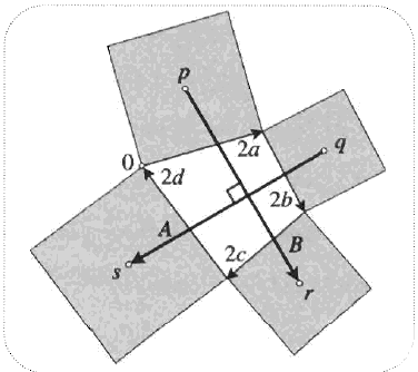
Theorem:The line segments joining the centers of opposite squares are perpendicular and of equal length.
定理:连接四边形各边外侧正方形中心的线段,互相垂直且长度相等。
Proof:
证明:
Let
2
a
,
2
b
,
2
c
,
2
d
2a, 2b, 2c, 2d
2a,2b,2c,2d be complex numbers running along the edges of the quadrilateral.
设
2
a
,
2
b
,
2
c
,
2
d
2a, 2b, 2c, 2d
2a,2b,2c,2d 为沿四边形各边的复数。
Condition for quadrilateral to close up is
四边形闭合的条件为
a + b + c + d = 0 a + b + c + d = 0 a+b+c+d=0
Let origin be at vertex where
2
a
2a
2a begins
设原点为
2
a
2a
2a 所在边的一个端点,则
p
=
a
+
i
a
p = a + ia
p=a+ia i.e.
a
a
a + (
a
a
a rotated though 90 degrees)
p
=
a
+
i
a
p = a + ia
p=a+ia,即
a
a
a 加上(旋转 90 度后的
a
a
a)
q
=
2
a
+
(
1
+
i
)
b
q = 2a + (1 + i) b
q=2a+(1+i)b
r
=
2
a
+
2
b
+
(
1
+
i
)
c
r = 2a + 2b + (1 + i) c
r=2a+2b+(1+i)c
s
=
2
a
+
2
b
+
2
c
+
(
1
+
i
)
d
s = 2a + 2b + 2c + (1 + i) d
s=2a+2b+2c+(1+i)d
A
=
s
−
q
A = s - q
A=s−q and
B
=
r
−
p
B = r - p
B=r−p
令
A
=
s
−
q
A = s - q
A=s−q,
B
=
r
−
p
B = r - p
B=r−p
we want to show that
A
A
A and
B
B
B are perpendicular and equal i.e.
B
=
i
A
B = iA
B=iA
需证明
A
A
A 与
B
B
B 互相垂直且长度相等,即
B
=
i
A
B = iA
B=iA
A + i B = ( a + b + c + d ) + i ( a + b + c + d ) = 0 A + iB = (a + b + c + d) + i (a + b + c + d) = 0 A+iB=(a+b+c+d)+i(a+b+c+d)=0
since
a
+
b
+
c
+
d
=
0
a + b + c + d = 0
a+b+c+d=0
因
a
+
b
+
c
+
d
=
0
a + b + c + d = 0
a+b+c+d=0,故上式成立。
This image, theorem, proof and everything is taken from Visual Complex Analysis by Tristan Needham.[One of the Best Books. Highly Recommended.]
该图像、定理、证明等所有内容,均取自特里斯坦・尼达姆(Tristan Needham)所著《可视化复分析》)。
answered Sep 24, 2010 at 6:42
Pratik Deoghare
I would simply say: “Wow!” (But this machine tells me that I must write at least 15 characters.)
我只想说:“哇!”(但系统提示我至少要写 15 个字符)。
– Agustí Roig
Commented Sep 24, 2010 at 7:24
+1 Very nice indeed! I guess I’ll have to buy Tristan Needham’s book.
+1 确实非常精彩!看来我得买本特里斯坦・尼达姆的书了。
– Adrián Barquero
Commented Sep 24, 2010 at 14:58
-
This shows up as well in Paul Lockhart’s video
保罗・洛克哈特(Paul Lockhart)的视频中也提到了这一点– isomorphismes
Commented Jun 14, 2014 at 13:51
A result that might be particularly suitable to students in a calculus sequence is complex partial fraction decomposition. Over the real numbers, you get denominators with both linear and quadratic factors, but over the complex numbers, algebraic closure means you only have to think about linear factors. For example, since
对修微积分课程的学生而言,一个特别合适的结论是 “复部分分式分解”。在实数域中,分式分解后的分母会同时包含一次和二次因式;但在复数域中,由于代数闭域性质,只需考虑一次因式。例如,由于
1 1 + x 2 = 1 2 ( 1 1 + i x + 1 1 − i x ) \frac {1}{1 + x^2} = \frac {1}{2} \left ( \frac {1}{1 + ix} + \frac {1}{1 - ix} \right) 1+x21=21(1+ix1+1−ix1)
it follows that
由此可推出
∫ 1 1 + x 2 d x = 1 2 ( i log ( 1 − i x ) − i log ( 1 + i x ) ) . \int \frac {1}{1 + x^2} dx = \frac {1}{2} \left ( i \log (1 - ix) - i \log (1 + ix) \right). ∫1+x21dx=21(ilog(1−ix)−ilog(1+ix)).
(It turns out that this function is just the arctangent in disguise.) So complex numbers give you a simple algorithm which you can use, in principle, to integrate any rational function. For example, in this recent math.SE thread it is shown that
(事实证明,该函数本质上就是反正切函数的另一种形式。)因此,复数提供了一种简单算法 —— 原则上,可利用该算法积分任何有理函数。例如,在近期的 math.SE 帖子中,已证明
1 1 − x n = 1 n ( ∑ k = 0 n − 1 1 1 − ζ k x ) \frac {1}{1 - x^n} = \frac {1}{n} \left ( \sum_{k=0}^{n - 1} \frac {1}{1 - \zeta^k x} \right) 1−xn1=n1(k=0∑n−11−ζkx1)
where
ζ
=
e
2
π
i
/
n
\zeta = e^{2\pi i /n}
ζ=e2πi/n is a primitive
n
t
h
n^{th}
nth root of unity. This implies that
其中
ζ
=
e
2
π
i
/
n
\zeta = e^{2\pi i /n}
ζ=e2πi/n 是本原
n
n
n 次单位根。这表明
∫ 1 1 − x n d x = 1 n ( ∑ k = 0 n − 1 − ζ − k log ( 1 − ζ k x ) ) . \int \frac {1}{1 - x^n} dx = \frac {1}{n} \left ( \sum_{k=0}^{n - 1} - \zeta^{-k} \log (1 - \zeta^k x) \right). ∫1−xn1dx=n1(k=0∑n−1−ζ−klog(1−ζkx)).
Not an integral most students would suspect is expressible in closed form! The analogous computation of
∫
1
1
+
x
n
d
x
\int \frac {1}{1 + x^n} dx
∫1+xn1dx would even allow you to express the sum
∑
k
=
0
∞
(
−
1
)
k
k
n
+
1
\sum_{k=0}^{\infty} \frac {(-1)^k}{k n + 1}
∑k=0∞kn+1(−1)k in closed form (which is just the definite integral from 0 to 1). These examples illustrate another application of the discrete Fourier transform, but the method I’m describing here is totally general.
这可不是大多数学生能想到的、可表示为闭式的积分!类似地,计算
∫
1
1
+
x
n
d
x
\int \frac {1}{1 + x^n} dx
∫1+xn1dx 甚至能让你将和式
∑
k
=
0
∞
(
−
1
)
k
k
n
+
1
\sum_{k=0}^{\infty} \frac {(-1)^k}{k n + 1}
∑k=0∞kn+1(−1)k 表示为闭式(该和式恰好是从 0 到 1 的定积分)。这些例子体现了离散傅里叶变换的另一应用,但我此处描述的方法具有完全的通用性。
edited Apr 13, 2017 at 12:20
3 revs
Qiaochu Yuan
- This is a great example; I remember T mentioning somewhere here that algorithms that have to be restricted to real variables are often clunky compared to algorithms that allow complexes.
这是个很棒的例子;我记得 T 曾在这里某处提到过:与允许使用复数的算法相比,局限于实变量的算法往往更繁琐。
– J. M. ain’t a mathematician
Commented Sep 20, 2010 at 22:10
I know of several ways to prove the Fundamental Theorem of Algebra using only basic tools from complex analysis. Suppose
P
(
z
)
P (z)
P(z) is a non-constant polynomial.
∣
P
(
z
)
∣
|P (z)|
∣P(z)∣ is large outside of a large disk, and inside that disk since
1
P
(
z
)
\frac {1}{P (z)}
P(z)1 is analytic,
1
∣
P
(
z
)
∣
\frac {1}{|P (z)|}
∣P(z)∣1 is bounded by the maximum it has on the boundary. Thus
1
P
(
z
)
\frac {1}{P (z)}
P(z)1 is a bounded analytic function on the whole plane so by Liouville’s Theorem it is constant, a contradiction. Thus
P
(
z
)
P (z)
P(z) has a zero somewhere.
我知道多种仅用复分析基础工具证明 “代数基本定理” 的方法。设
P
(
z
)
P (z)
P(z) 为非零次多项式:在大圆盘外部,
∣
P
(
z
)
∣
|P (z)|
∣P(z)∣ 的值很大;在圆盘内部,由于
1
P
(
z
)
\frac {1}{P (z)}
P(z)1 是解析函数,
1
∣
P
(
z
)
∣
\frac {1}{|P (z)|}
∣P(z)∣1 的值被其在边界上的最大值所界定。因此,
1
P
(
z
)
\frac {1}{P (z)}
P(z)1 是全平面上的有界解析函数,根据刘维尔定理(Liouville’s Theorem),它必为常数 —— 这与
P
(
z
)
P (z)
P(z) 是非零次多项式矛盾。故
P
(
z
)
P (z)
P(z) 必有零点。
This really only uses the fact that polynomials are analytic, and analytic functions satisfy the maximum principle. Liouville’s Theorem takes a little more work, but should be covered in any first complex analysis course.
该证明实际上仅利用了两个事实:多项式是解析的,以及解析函数满足最大值原理。刘维尔定理的证明稍复杂些,但任何一门复分析入门课程都应会讲解。
answered Sep 20, 2010 at 16:59
Matt
Yet another example close to my heart: one of the hundred-dollar hundred-digit problems asked for the value of
再举一个我格外喜欢的例子:“百美元百位数难题” 中的一道题,要求计算
I = lim ε → 0 ∫ ε 1 1 t cos ( ln t t ) d t I = \lim_{\varepsilon \to 0} \int_{\varepsilon}^{1} \frac {1}{t} \cos\left ( \frac {\ln t}{t} \right) dt I=ε→0lim∫ε1t1cos(tlnt)dt
One solution was to transform it into an oscillatory integral with infinite limit, but the slickest solution to this problem was to use a contour in the complex plane that side-stepped the numerical difficulties with having an oscillatory integrand:
一种解法是将其转化为无穷限振荡积分,但最简洁的解法是利用复平面中的积分路径,避开振荡被积函数带来的数值计算难题:
I = ℜ ( ∫ 0 1 t i t − 1 d t ) I = \Re \left ( \int_{0}^{1} t^{\frac {i}{t} - 1} dt \right) I=ℜ(∫01tti−1dt)
and by using an appropriate contour, even the humble trapezoidal rule suffices to handle the integral.
通过选择合适的积分路径,即便用简单的梯形法则(trapezoidal rule),也能处理这个积分。
answered Sep 19, 2010 at 2:13
J. M. ain’t a mathematician
-
P.S. The Hadamard quote Mariano gave in the comments is in fact mentioned in the chapter of the book about this problem set.
– J. M. ain’t a mathematician
Commented Sep 19, 2010 at 2:41
附言:Mariano 在评论中引用的阿达马名言,实际上在该书关于这套难题的章节中也有提及。
——J. M. ain’t a mathematician
2010 年 9 月 19 日 2:41 评论 -
For a Mathematica demonstration, compare
若用 Mathematica(数学软件)演示,可对比以下两段代码的运行结果:- 振荡积分方法
Timing [NIntegrate [ProductLog'[t] Cos [t], {t, 0, Infinity}, Method -> Oscillatory, WorkingPrecision -> 20]]
and - 复路径积分方法
Timing [Re [NIntegrate [(t + I t (1 - t))^(I/(t + I t (1 - t)) - 1)(1 + I (1 - 2t)), {t, 0, 1}, WorkingPrecision -> 20]]]
– J. M. ain’t a mathematician
Commented Sep 19, 2010 at 3:21 - 振荡积分方法
There are tons of applications of complex numbers in places you would not expect. Number theory is one, for example. This example is fromThe Art and Craft of Problem Solvingby Zeitz.
复数在许多意想不到的领域都有大量应用,数论就是其中之一。以下例子取自蔡茨(Zeitz)所著的《解题的艺术与技巧》。
Proposition: If
m
m
m and
n
n
n are integers that can be written as the sum of two squares, then
m
n
mn
mn can also be written as the sum of two squares.
命题:若整数
m
m
m 和
n
n
n 均可表示为两个平方数之和,则
m
n
mn
mn 也可表示为两个平方数之和。
Proof: Let
m
=
a
2
+
b
2
m = a^2 + b^2
m=a2+b2 and
n
=
c
2
+
d
2
n = c^2 + d^2
n=c2+d2 and define
z
=
(
a
+
b
i
)
(
c
+
d
i
)
z = (a + bi)(c + di)
z=(a+bi)(c+di). Then
∣
z
∣
2
=
∣
a
+
b
i
∣
2
∣
c
+
d
i
∣
2
=
m
n
|z|^2 = |a + bi|^2 |c + di|^2 = mn
∣z∣2=∣a+bi∣2∣c+di∣2=mn. Since
ℜ
(
z
)
=
a
c
−
b
d
\Re (z) = ac - bd
ℜ(z)=ac−bd and
ℑ
(
z
)
=
b
c
+
a
d
\Im (z) = bc + ad
ℑ(z)=bc+ad are both integers and
∣
z
∣
2
|z|^2
∣z∣2 equals the sum of the squares of its real and imaginary components, then
∣
z
∣
2
=
m
n
|z|^2 = mn
∣z∣2=mn is the sum of two squares.
证明:设
m
=
a
2
+
b
2
m = a^2 + b^2
m=a2+b2,
n
=
c
2
+
d
2
n = c^2 + d^2
n=c2+d2,定义
z
=
(
a
+
b
i
)
(
c
+
d
i
)
z = (a + bi)(c + di)
z=(a+bi)(c+di)。则
∣
z
∣
2
=
∣
a
+
b
i
∣
2
∣
c
+
d
i
∣
2
=
m
n
|z|^2 = |a + bi|^2 |c + di|^2 = mn
∣z∣2=∣a+bi∣2∣c+di∣2=mn。由于
ℜ
(
z
)
=
a
c
−
b
d
\Re (z) = ac - bd
ℜ(z)=ac−bd(实部)和
ℑ
(
z
)
=
b
c
+
a
d
\Im (z) = bc + ad
ℑ(z)=bc+ad(虚部)均为整数,且
∣
z
∣
2
|z|^2
∣z∣2 等于其实部与虚部的平方和,因此
∣
z
∣
2
=
m
n
|z|^2 = mn
∣z∣2=mn 可表示为两个平方数之和。
edited Sep 20, 2010 at 19:13
2 revs
Lukas Owens
I just remembered something that at the moment seemed pretty nice to me. Usually in an elementary number theory course one is taught that the integer solutions to the diophantine equation
x
2
+
y
2
=
z
2
x^2 + y^2 = z^2
x2+y2=z2 are given by the formulas
x
=
a
2
−
b
2
x = a^2 - b^2
x=a2−b2,
y
=
2
a
b
y = 2ab
y=2ab and
z
=
a
2
+
b
2
z = a^2 + b^2
z=a2+b2. By working in a naive way in the ring of Gaussian integers
Z
[
i
]
=
{
a
+
b
i
∣
a
,
b
∈
Z
}
\mathbb {Z}[i] = \{ a + bi \mid a, b \in \mathbb {Z} \}
Z[i]={a+bi∣a,b∈Z} one can get these formulas without much effort.
我刚想起一件当时觉得很精彩的事:在基础数论课程中,通常会教到丢番图方程
x
2
+
y
2
=
z
2
x^2 + y^2 = z^2
x2+y2=z2(勾股方程)的整数解由公式
x
=
a
2
−
b
2
x = a^2 - b^2
x=a2−b2、
y
=
2
a
b
y = 2ab
y=2ab、
z
=
a
2
+
b
2
z = a^2 + b^2
z=a2+b2 给出。若在高斯整数环
Z
[
i
]
=
{
a
+
b
i
∣
a
,
b
∈
Z
}
\mathbb {Z}[i] = \{ a + bi \mid a, b \in \mathbb {Z} \}
Z[i]={a+bi∣a,b∈Z} 中简单运算,无需过多步骤就能推出这些公式。
We factor the equation as
将方程因式分解为
( x + i y ) ( x − i y ) = z 2 (x + iy)(x - iy) = z^2 (x+iy)(x−iy)=z2
Then since the right hand side is a square, the two factors on the left must be squares of numbers in
Z
[
i
]
\mathbb {Z}[i]
Z[i] so for instance
由于右侧是平方数,左侧的两个因式必为
Z
[
i
]
\mathbb {Z}[i]
Z[i] 中的平方数,因此不妨设
x
+
i
y
=
(
a
+
b
i
)
2
x + iy = (a + bi)^2
x+iy=(a+bi)2
and squaring this gives
将右侧展开可得
x
+
i
y
=
a
2
−
b
2
+
2
a
b
i
x + iy = a^2 - b^2 + 2abi
x+iy=a2−b2+2abi
Now equating real and imaginary parts shows that
x
=
a
2
−
b
2
x = a^2 - b^2
x=a2−b2 and
y
=
2
a
b
y = 2ab
y=2ab. From this one easily gets
z
=
a
2
+
b
2
z = a^2 + b^2
z=a2+b2. Of course all of these manipulations need some more details but it would make for a nice example after the formulas have been derived in the usual way (without complex numbers).
比较等式两边的实部和虚部,可得
x
=
a
2
−
b
2
x = a^2 - b^2
x=a2−b2、
y
=
2
a
b
y = 2ab
y=2ab。由此可轻松推出
z
=
a
2
+
b
2
z = a^2 + b^2
z=a2+b2。当然,这些运算还需补充一些细节,但在(不借助复数的)常规方法推导出公式后,这会是一个很好的补充例子。
edited Sep 20, 2010 at 23:38
2 revs
Adrián Barquero
- Squaring
(
a
+
b
i
)
2
=
a
2
−
b
2
+
2
a
b
i
(a + bi)^2 = a^2 - b^2 + 2abi
(a+bi)2=a2−b2+2abi gives the result in an easier way.
直接将 ( a + b i ) 2 = a 2 − b 2 + 2 a b i (a + bi)^2 = a^2 - b^2 + 2abi (a+bi)2=a2−b2+2abi 展开,能更简单地得到结果。
– u8y7541
Commented Dec 18, 2017 at 6:07
- 复数 | 存在意义 / 实际应用(篇 1 )-优快云博客
https://blog.youkuaiyun.com/u013669912/article/details/154277501
via:
- soft question - Demystifying complex numbers
https://mathoverflow.net/questions/30156/demystifying-complex-numbers - Interesting results easily achieved using complex numbers
https://math.stackexchange.com/questions/4961/interesting-results-easily-achieved-using-complex-numbers


 被折叠的 条评论
为什么被折叠?
被折叠的 条评论
为什么被折叠?
 到【灌水乐园】发言


