


注:本文为英文引文,机翻未校。
如有内容异常,请看原文。
因 csdn 篇幅字符限制,分为两篇。
3 Design of estimators for stochastic hybrid systems
随机混合系统的估计器设计
Having established conditions for the observability of stochastic linear hybrid systems, we would like to design estimators for those observable systems, and also quantify values of system parameters that would guarantee performance (exponential convergence, in our case). We extend the design methods proposed by Balluchi et al. [6] for hybrid systems with continuous-time, continuous state dynamics to encompass discrete-time stochastic hybrid systems.
在建立随机线性混合系统的可观测性条件后,我们希望为这些可观测系统设计估计器,并量化系统参数的取值,以保证估计器的性能(本文中为指数收敛)。我们将 Balluchi 等人(文献[6])提出的适用于连续时间、连续状态动力学混合系统的估计器设计方法推广到离散时间随机混合系统中。
A hybrid estimator finds estimates
q
^
\hat{q}
q^ and
x
^
\hat{x}
x^ for the current discrete state
q
q
q and the continuous state
x
x
x respectively. In this section, we first describe the structure of the hybrid estimator, and then analyze the continuous component of the estimator in detail to obtain bounds on the time between discrete transitions of state which would guarantee exponential convergence of our hybrid estimator. Throughout this paper, all norms, unless specified otherwise, are 2-norms.
混合估计器用于估计当前离散状态
q
q
q 和连续状态
x
x
x 的估计值
q
^
\hat{q}
q^ 和
x
^
\hat{x}
x^ 。在本节中,我们首先描述混合估计器的结构,然后详细分析估计器的连续部分,以确定离散切换时间间隔的界,从而保证混合估计器的指数收敛性。在本文中,除非另有说明,所有范数均为 2-范数。
Definition 5 (Exponential convergence of a hybrid estimator) Given a hybrid system
H
H
H with
N
N
N discrete modes, we say that a hybrid estimator is exponentially convergent if its discrete state estimate
q
^
\hat{q}
q^ exhibits correct identification of the discrete-state transition sequence of the original system after a finite number of steps; the continuous state estimate at any instant has a unique mean and convergent covariance; and the mean of the estimation error,
ζ
ˉ
=
E
[
x
^
−
x
]
\bar{\zeta}=E[\hat{x}-x]
ζˉ=E[x^−x] converges exponentially to the set
∥
ζ
ˉ
∥
≤
M
0
\|\bar{\zeta}\| \leq M_{0}
∥ζˉ∥≤M0 with a rate of convergence
μ
\mu
μ , where
M
0
M_0
M0 is the steady-state error bound, and
∣
μ
∣
<
1
|\mu|<1
∣μ∣<1 . In other words, the estimator is convergent if for any switching time
k
i
k_{i}
ki ,
定义 5(混合估计器的指数收敛性) 对于具有
N
N
N 个离散模式的混合系统
H
H
H ,若混合估计器满足以下条件,则称其具有指数收敛性:其离散状态估计值
q
^
\hat{q}
q^ 能在有限步内正确识别原始系统的离散状态切换序列;任意时刻的连续状态估计值具有唯一均值和收敛的协方差;估计误差的均值
ζ
ˉ
=
E
[
x
^
−
x
]
\bar{\zeta}=E[\hat{x}-x]
ζˉ=E[x^−x] 以收敛速率
μ
\mu
μ 指数收敛到集合
∥
ζ
ˉ
∥
≤
M
0
\|\bar{\zeta}\| \leq M_{0}
∥ζˉ∥≤M0 (其中
M
0
M_0
M0 为稳态误差界,且
∣
μ
∣
<
1
|\mu|<1
∣μ∣<1 )。换句话说,估计器是收敛的,若对于任意切换时刻
k
i
k_{i}
ki ,满足:
q
^
k
=
q
k
,
∀
k
>
K
,
K
∈
N
+
∥
ζ
ˉ
k
∥
≤
μ
(
k
−
k
i
)
∥
ζ
ˉ
k
i
∥
+
M
0
,
∀
k
>
k
i
\begin{align} \hat{q}_k & \; = \; q_k, \forall k > K, K \in \mathbb{N}^+ \tag{11} \\ \|\bar{\zeta}_k\| & \; \leq \; \mu^{(k-k_i)}\|\bar{\zeta}_{k_i}\| + M_0, \forall k > k_i \tag{12} \end{align}
q^k∥ζˉk∥=qk,∀k>K,K∈N+≤μ(k−ki)∥ζˉki∥+M0,∀k>ki(11)(12)
3.1 Structure of the hybrid estimator
混合估计器的结构
We design the hybrid estimator as a combination of a discrete observer to detect the discrete state switches, and an estimator to estimate the continuous dynamics, as proposed in [6]. In the rest of this paper, we assume that we have a discrete observer that correctly identifies the discrete state, either immediately after a switch takes place, or with a known time delay
Δ
\Delta
Δ after a discrete transition. A discrete observer could be constructed using a bank of
N
N
N estimators as a residual generator [1,6] – even in this case, we could further increase the probability of correct discrete-state identification by enforcing a decision time delay
Δ
\Delta
Δ on the discrete observer. This would be possible only if the system were observable in the sense of a stochastic hybrid system, as explained earlier. In this section, we design a least-squares estimator in the form of Kalman filters for the continuous state estimate. Although the underlying system in [6] is continuous-time and deterministic, the design methodology of [6] adapts well to discrete-time stochastic hybrid systems, as we show here.
我们设计的混合估计器由离散观测器和连续状态估计器组成,其中离散观测器用于检测离散状态切换,连续状态估计器用于估计连续动力学过程(参见文献[6])。在本文后续部分,我们假设存在一个离散观测器,能够在离散切换发生后立即或在已知时间延迟
Δ
\Delta
Δ 后正确识别离散状态。即使在这种情况下,我们也可以通过在离散观测器上施加决策时间延迟
Δ
\Delta
Δ,进一步提高正确识别离散状态的概率。这只有在系统以随机混合系统的意义下是可观测的情况下才可能实现,如前文所述。在本节中,我们设计了一种以卡尔曼滤波器形式呈现的最小二乘估计器,用于估计连续状态。尽管文献[6] 中的底层系统是连续时间确定性系统,但文献[6] 的设计方法可以很好地适应离散时间随机混合系统,正如我们在本文中所展示的那样。
3.2 Discrete-time Kalman filter
离散时间卡尔曼滤波器
We consider a hybrid system of the form described in Eq.(1). For the sake of simplicity of notation, we replace
A
(
q
k
)
A(q_{k})
A(qk) and
C
(
q
k
)
C(q_{k})
C(qk) with
A
l
A_l
Al and
C
l
C_{l}
Cl , where
l
∈
{
1
,
.
.
.
,
N
}
l \in \{1, ..., N\}
l∈{1,...,N} . We can then write the equations for the least-square estimator of a linear stochastic system as
考虑如式 (1) 所示形式的混合系统。为了简化符号,我们将
A
(
q
k
)
A(q_{k})
A(qk) 和
C
(
q
k
)
C(q_{k})
C(qk) 分别替换为
A
l
A_l
Al 和
C
l
C_{l}
Cl ,其中
l
∈
{
1
,
.
.
.
,
N
}
l \in \{1, ..., N\}
l∈{1,...,N} 。于是,线性随机系统的最小二乘估计器方程可以表示为:
x ^ k + 1 = ( A l − K P , k , l C l ) x ^ k + K P , k , l y k , k ≥ 0 (13) \hat{x}_{k+1}=\left(A_{l}-K_{P,k,l} C_{l}\right) \hat{x}_{k}+K_{P,k,l} y_{k}, \quad k \geq 0\tag{13} x^k+1=(Al−KP,k,lCl)x^k+KP,k,lyk,k≥0(13)
where
l
l
l is the estimated discrete state, and
K
P
,
k
,
l
K_{P,k,l}
KP,k,l is the optimal Kalman filter gain for mode
l
l
l , given by
其中,
l
l
l 是估计的离散状态,
K
P
,
k
,
l
K_{P,k,l}
KP,k,l 是模式
l
l
l 下的最优卡尔曼滤波器增益,具体为:
K P , k , l = A l P k C l T ( C l P k C l T + R l ) − 1 (14) K_{P,k,l} = A_l P_k C_l^T \left(C_l P_k C_l^T + R_l\right)^{-1} \tag{14} KP,k,l=AlPkClT(ClPkClT+Rl)−1(14)
and
P
k
P_{k}
Pk satisfies the discrete Riccati recursion
并且
P
k
P_{k}
Pk 满足离散黎卡提递推方程:
P k + 1 = A l P k A l T + Q l − K P , k , l ( R l + C l P k C l T ) K P , k , l T , P ( 0 ) ≜ Π 0 (15) P_{k+1}=A_{l} P_{k} A_{l}^{T}+Q_{l}-K_{P,k,l}\left(R_{l}+C_{l} P_{k} C_{l}^{T}\right) K_{P,k,l}^{T}, \quad P(0) \triangleq \Pi_{0} \tag{15} Pk+1=AlPkAlT+Ql−KP,k,l(Rl+ClPkClT)KP,k,lT,P(0)≜Π0(15)
where
Q
l
=
ρ
(
q
l
)
I
Q_l = \rho(q_l)I
Ql=ρ(ql)I and
R
l
=
σ
(
q
l
)
I
R_l = \sigma(q_l)I
Rl=σ(ql)I .
其中,
Q
l
=
ρ
(
q
l
)
I
Q_l = \rho(q_l)I
Ql=ρ(ql)I 和
R
l
=
σ
(
q
l
)
I
R_l = \sigma(q_l)I
Rl=σ(ql)I 。
Theorem 2 ([13]): The Discrete Algebraic Riccati Equation (DARE) has a stabilizing solution that is unique if and only if
定理 2(文献[13]):离散代数黎卡提方程(DARE)有唯一的稳定解,当且仅当满足以下条件:
{
A
l
,
C
l
}
is detectable
{
A
l
,
C
l
}
是可检测的
{
A
l
,
Q
l
1
/
2
}
is controllable on the unit circle.
{
A
l
,
Q
l
1
/
2
}
在单位圆上是可控的。
\begin{align} \{A_l, C_l\} \text{ is detectable} & \quad \{A_l, C_l\} \text{ 是可检测的} \tag{16} \\ \{A_l, Q_l^{1/2}\} \text{ is controllable on the unit circle.} & \quad \{A_l, Q_l^{1/2}\} \text{ 在单位圆上是可控的。} \tag{17} \end{align}
{Al,Cl} is detectable{Al,Ql1/2} is controllable on the unit circle.{Al,Cl} 是可检测的{Al,Ql1/2} 在单位圆上是可控的。(16)(17)
Any such solution is positive definite.
任何这样的解都是正定的。
If these conditions are satisfied for every discrete state
i
∈
{
1
…
N
}
i \in \{1 \ldots N\}
i∈{1…N}, we can design a bank of
N
N
N steady-state, exponentially convergent Kalman filters to estimate the continuous state of the system.
如果这些条件对每个离散状态
i
∈
{
1
…
N
}
i \in \{1 \ldots N\}
i∈{1…N} 都满足,我们可以设计一组
N
N
N 个稳态、指数收敛的卡尔曼滤波器来估计系统的连续状态。
We can then show that, for a given discrete state
i
i
i, correctly identified,
我们然后可以展示,对于一个给定的离散状态
i
i
i,正确识别,
x ^ k + 1 = ( A l − K l C l ) x ^ k + K l y k ζ ^ k + 1 = ( A l − K l C l ) ζ ^ k \begin{align} \hat{x}_{k+1} &= (A_l - K_l C_l) \hat{x}_k + K_l y_k \tag{18} \\ \hat{\zeta}_{k+1} &= (A_l - K_l C_l) \hat{\zeta}_k \tag{19} \end{align} x^k+1ζ^k+1=(Al−KlCl)x^k+Klyk=(Al−KlCl)ζ^k(18)(19)
Clearly,
ζ
^
\hat{\zeta}
ζ^ is exponentially convergent if
(
A
l
−
K
l
C
l
)
is stable
k
(20)
(A_l - K_l C_l)\; \text{is stable} k \tag{20}
(Al−KlCl)is stablek(20)
显然,如果
(
A
l
−
K
l
C
l
)
(A_l - K_l C_l)
(Al−KlCl) 是稳定的,
ζ
^
\hat{\zeta}
ζ^ 是指数收敛的。
3.3 Error dynamics
误差动力学
In this section, we follow the methodology of [6] to determine the evolution of the estimation error across the discrete transition sequence. Let us consider two consequent discrete transitions of
H
H
H , occurring at times
k
i
k_{i}
ki and
k
i
+
1
k_{i+1}
ki+1 . Suppose the transition at time
k
i
+
1
k_{i+1}
ki+1 was from discrete state
m
m
m to
l
l
l , and was detected at time
k
i
+
1
′
k_{i+1}'
ki+1′ such that
k
i
+
1
′
−
k
i
+
1
≤
Δ
k_{i+1}' - k_{i+1} \leq \Delta
ki+1′−ki+1≤Δ . Similarly, the previous transition at time
k
i
k_i
ki was detected at time
k
i
′
k_i'
ki′ such that
k
i
′
−
k
i
≤
Δ
k_i' - k_i \leq \Delta
ki′−ki≤Δ . This is illustrated in Fig.(1).
在本节中,我们遵循文献[6] 的方法,研究估计误差在离散切换序列中的演变。考虑混合系统
H
H
H 的两个连续离散切换,分别发生在时刻
k
i
k_{i}
ki 和
k
i
+
1
k_{i+1}
ki+1 。假设在时刻
k
i
+
1
k_{i+1}
ki+1 发生的离散切换是从离散状态
m
m
m 切换到离散状态
l
l
l ,并且在时刻
k
i
+
1
′
k_{i+1}'
ki+1′ 被检测到,满足
k
i
+
1
′
−
k
i
+
1
≤
Δ
k_{i+1}' - k_{i+1} \leq \Delta
ki+1′−ki+1≤Δ 。类似地,之前的切换发生在时刻
k
i
k_i
ki ,并在时刻
k
i
′
k_i'
ki′ 被检测到,满足
k
i
′
−
k
i
≤
Δ
k_i' - k_i \leq \Delta
ki′−ki≤Δ 。如图 1 所示。
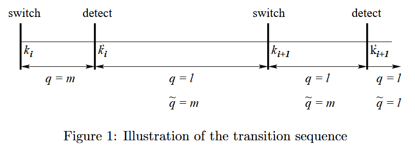
Figure 1: Illustration of the transition sequence
图 1:切换序列示意图
We are interested in the region
k
∈
{
k
i
′
,
k
i
′
+
1
,
.
.
.
,
k
i
+
1
′
}
k \in \{k_{i}', k_{i}'+1, ..., k_{i+1}'\}
k∈{ki′,ki′+1,...,ki+1′} . Since we assume that by time-step
k
i
′
k_{i}'
ki′ the discrete state has been identified correctly, for the exponential convergence of the estimation error on
k
i
′
k_{i'}
ki′ to
k
i
+
1
′
k_{i+1}'
ki+1′ :
我们关注的区域是
k
∈
{
k
i
′
,
k
i
′
+
1
,
.
.
.
,
k
i
+
1
′
}
k \in \{k_{i}', k_{i}'+1, ..., k_{i+1}'\}
k∈{ki′,ki′+1,...,ki+1′} 。由于我们假设在时刻
k
i
′
k_{i}'
ki′ 已经正确识别了离散状态,因此为了保证估计误差从
k
i
′
k_{i'}
ki′ 到
k
i
+
1
′
k_{i+1}'
ki+1′ 的指数收敛性:
- The error converges exponentially between
k
i
′
k_{i}'
ki′ and
k
i
+
1
k_{i+1}
ki+1 ; and
估计误差在 k i ′ k_{i}' ki′ 至 k i + 1 k_{i+1} ki+1 区间内指数收敛; - The error divergence between
k
i
+
1
k_{i+1}
ki+1 and
k
i
+
1
′
k_{i+1}'
ki+1′ due to wrong discrete state estimation does not upset the exponential convergence of the error on
k
i
′
k_{i}'
ki′ to
k
i
+
1
′
k_{i+1}'
ki+1′ .
在 k i + 1 k_{i+1} ki+1 至 k i + 1 ′ k_{i+1}' ki+1′ 区间内,由离散状态估计错误导致的误差发散,不会破坏估计误差在 k i ′ k_{i}' ki′ 至 k i + 1 ′ k_{i+1}' ki+1′ 区间内的指数收敛性。
Following the methodology of [6], dividing the time interval between
k
i
′
k_{i}'
ki′ and
k
i
+
1
′
k_{i+1}'
ki+1′ into two regions, we get error dynamics of the form
按照文献[6] 的方法,将区间
k
i
′
k_{i}'
ki′ 至
k
i
+
1
′
k_{i+1}'
ki+1′ 划分为两个部分,得到误差动力学方程如下:
ζ ˉ k + 1 = ( A m − K m C m ) ζ ˉ k k ∈ { k i ′ , … , k i + 1 − 1 } ζ ˉ k + 1 = ( A m − K m C m ) ζ ˉ k + [ ( A m − A l ) − K m ( C m − C l ) ] x ˉ k k ∈ { k i + 1 , … , k i + 1 ′ − 1 } \begin{align} \bar{\zeta}_{k+1} &= (A_m - K_m C_m) \bar{\zeta}_k \tag{21} \\ &k \in \{k_i', \ldots, k_{i+1} - 1\} \nonumber \\ \bar{\zeta}_{k+1} &= (A_m - K_m C_m) \bar{\zeta}_k + [(A_m - A_l) - K_m (C_m - C_l)] \bar{x}_k \tag{22} \\ &k \in \{k_{i+1}, \ldots, k_{i+1}' - 1\} \nonumber \end{align} ζˉk+1ζˉk+1=(Am−KmCm)ζˉkk∈{ki′,…,ki+1−1}=(Am−KmCm)ζˉk+[(Am−Al)−Km(Cm−Cl)]xˉkk∈{ki+1,…,ki+1′−1}(21)(22)
where
x
ˉ
=
E
[
x
]
\bar{x}=E[x]
xˉ=E[x] . The second term in the second equation of Eq.(22) arises because a Kalman filter designed for the discrete state
m
m
m is being used to estimate the dynamics of the discrete state
l
l
l . Combining the two equations in Eq.(22), we express the error dynamics by
其中,
x
ˉ
=
E
[
x
]
\bar{x}=E[x]
xˉ=E[x] 。式 (22) 中第二个方程的第二项源于:实际使用为离散状态
m
m
m 设计的卡尔曼滤波器,去估计离散状态
l
l
l 的动力学过程。联立式 (22) 中的两个方程,误差动力学可表示为:
ζ ˉ k + 1 = ( A m − K m C m ) ζ ˉ k + u k , k ∈ { k i ′ , … , k i + 1 ′ − 1 } (23) \bar{\zeta}_{k+1} = (A_m - K_m C_m) \bar{\zeta}_k + u_k, \quad k \in \{k'_i, \ldots, k'_{i+1} - 1\} \tag{23} ζˉk+1=(Am−KmCm)ζˉk+uk,k∈{ki′,…,ki+1′−1}(23)
where
其中:
u k = { 0 , k ∈ { k i ′ , … , k i + 1 − 1 } ( ( A m − A l ) − K m ( C m − C l ) ) x ‾ k , k ∈ { k i + 1 , . . . , k i + 1 ′ − 1 } (24) u_{k}=\left\{ \begin{array}{ll} 0, & k\in \{ k_{i}^{\prime },\dots ,k_{i+1}-1\} \\ \left( (A_{m}-A_{l})-K_{m}(C_{m}-C_{l})\right)\overline {x}_{k}, & k\in \left\{ k_{i+1}, ..., k_{i+1}'-1\right\} \end{array} \right.\tag{24} uk={0,((Am−Al)−Km(Cm−Cl))xk,k∈{ki′,…,ki+1−1}k∈{ki+1,...,ki+1′−1}(24)
From this, we get
由此可得到:
ζ ˉ k + 1 = ( A m − K m C m ) k + 1 − k i ′ ζ ˉ k i ′ + [ ( A m − K m C m ) k − k i ′ … I ] [ u k i ′ ⋮ u k ] ∥ ζ ˉ k + 1 ∥ = ∥ ( A m − K m C m ) k + 1 − k i ′ ζ ˉ k i ′ + [ ( A m − K m C m ) k − k i ′ … I ] [ u k i ′ ⋮ u k ] ∥ \begin{align} \bar{\zeta}_{k+1} &= (A_m - K_m C_m)^{k+1-k_i'} \bar{\zeta}_{k_i'} + \left[(A_m - K_m C_m)^{k-k_i'} \ldots I \right] \begin{bmatrix} u_{k_i'} \\ \vdots \\ u_k \end{bmatrix} \tag{25} \\ \|\bar{\zeta}_{k+1}\| &= \left\| (A_m - K_m C_m)^{k+1-k_i'} \bar{\zeta}_{k_i'} + \left[(A_m - K_m C_m)^{k-k_i'} \ldots I \right] \begin{bmatrix} u_{k_i'} \\ \vdots \\ u_k \end{bmatrix} \right\| \tag{26} \end{align} ζˉk+1∥ζˉk+1∥=(Am−KmCm)k+1−ki′ζˉki′+[(Am−KmCm)k−ki′…I] uki′⋮uk = (Am−KmCm)k+1−ki′ζˉki′+[(Am−KmCm)k−ki′…I] uki′⋮uk (25)(26)
This gives us
这给出了:
∥ ζ ˉ k + 1 ∥ = ∥ ( A m − K m C m ) k + 1 − k i ′ ζ ˉ k i ′ + ∑ l = 0 k − k i ′ ( A m − K m C m ) k − k i ′ − l u k i ′ + l ∥ , k ∈ { k i + 1 , … , k i + 1 ′ − 1 } ≤ ∥ ( A m − K m C m ) k + 1 − k i ′ ζ ˉ k i ′ ∥ + ∥ ∑ l = 0 k − k i ′ ( A m − K m C m ) k − k i ′ − l u k i ′ + l ∥ , k ∈ { k i + 1 , … , k i + 1 ′ − 1 } \begin{align} \|\bar{\zeta}_{k+1}\| &= \left\| (A_m - K_m C_m)^{k+1-k_i'} \bar{\zeta}_{k_i'} + \sum_{l=0}^{k-k_i'} (A_m - K_m C_m)^{k-k_i'-l} u_{k_i'+l} \right\|, \, k \in \{k_{i+1}, \ldots, k_{i+1}' - 1\} \tag{27} \\ &\leq \left\| (A_m - K_m C_m)^{k+1-k_i'} \bar{\zeta}_{k_i'} \right\| + \left\| \sum_{l=0}^{k-k_i'} (A_m - K_m C_m)^{k-k_i'-l} u_{k_i'+l} \right\|, \, k \in \{k_{i+1}, \ldots, k_{i+1}' - 1\} \tag{28} \end{align} ∥ζˉk+1∥= (Am−KmCm)k+1−ki′ζˉki′+l=0∑k−ki′(Am−KmCm)k−ki′−luki′+l ,k∈{ki+1,…,ki+1′−1}≤ (Am−KmCm)k+1−ki′ζˉki′ + l=0∑k−ki′(Am−KmCm)k−ki′−luki′+l ,k∈{ki+1,…,ki+1′−1}(27)(28)
Lemma 4 Given a matrix
A
∈
R
n
×
n
A \in \mathbb{R}^{n \times n}
A∈Rn×n with all distinct eigenvalues, there exists a constant
k
(
A
)
>
0
k(A) > 0
k(A)>0 such that
∥
A
t
∥
≤
k
(
A
)
α
(
A
)
t
\|A^t\| \leq k(A) \alpha(A)^t
∥At∥≤k(A)α(A)t for all
t
≥
0
t \geq 0
t≥0 ,
引理 4 对于所有特征值互不相同的矩阵
A
∈
R
n
×
n
A \in \mathbb{R}^{n \times n}
A∈Rn×n ,存在常数
k
(
A
)
>
0
k(A) > 0
k(A)>0 ,使得对所有
t
≥
0
t \geq 0
t≥0 ,均有
∥
A
t
∥
≤
k
(
A
)
α
(
A
)
t
\|A^t\| \leq k(A) \alpha(A)^t
∥At∥≤k(A)α(A)t 。
∥
A
t
∥
≤
k
(
A
)
α
t
(
A
)
,
∀
t
≥
0
(29)
\|A^t\| \leq k(A) \alpha^t(A), \quad \forall t \geq 0 \tag{29}
∥At∥≤k(A)αt(A),∀t≥0(29)
where
α
(
A
)
\alpha(A)
α(A) is the maximal absolute value of the eigenvalues of
A
A
A , and
k
(
A
)
k(A)
k(A) is the condition number of
A
A
A under the inverse, where
Q
−
1
A
Q
=
J
Q^{-1} A Q=J
Q−1AQ=J , the Jordan canonical form.
其中,
α
(
A
)
\alpha(A)
α(A) 是矩阵
A
A
A 所有特征值的最大绝对值;
k
(
A
)
k(A)
k(A) 是矩阵
A
A
A 的逆条件数(矩阵
A
A
A 经相似变换化为若尔当标准形
J
J
J ,即
Q
−
1
A
Q
=
J
Q^{-1} A Q = J
Q−1AQ=J ,
k
(
A
)
k(A)
k(A) 由该变换定义)。
Proof: The proof follows that for the continuous-time case ( [6], [14]). From this we can show that for
t
≥
0
t \geq 0
t≥0 , if
m
m
m is the size of the largest Jordan block of
A
A
A ,
证明:证明过程与连续时间情形类似(文献[6], [14])。由此可证明,对于
t
≥
0
t \geq 0
t≥0 ,若
m
m
m 是矩阵
A
A
A 最大若尔当块的阶数,则:
∥ A t ∥ ≤ m k ( A ) α t ( A ) max t r α r ( A ) , 0 ≤ r ≤ m − 1 (30) \|A^t\| \leq mk(A)\alpha^t(A) \max \frac{t^r}{\alpha^r(A)}, \quad 0 \leq r \leq m-1 \tag{30} ∥At∥≤mk(A)αt(A)maxαr(A)tr,0≤r≤m−1(30)
When
A
A
A has all distinct eigenvalues, this reduces to Eq.(29). □
当矩阵
A
A
A 所有特征值互不相同时,可简化为式 (29)。□
Further simplification of Eq.(28) using Lemma 4 gives us
利用引理 4 对式 (28) 进一步化简,可得:
∥ ζ ˉ k + 1 ∥ ≤ k ( A m − C m ) [ α ( A m − K m C m ) ] k + 1 − k i ′ ∥ ζ ˉ k i ′ ∥ + k ( A m − C m ) max ∥ u k ∥ ( k − k i + 1 ) , k ∈ { k i + 1 , … , k i + 1 ′ } \begin{align} \|\bar{\zeta}_{k+1}\| \leq & \quad k(A_m - C_m)[\alpha(A_m - K_m C_m)]^{k+1-k_i'} \|\bar{\zeta}_{k_i'}\| \nonumber \\ & + \, k(A_m - C_m) \max \|u_k\| \, (k - k_{i+1}), \, k \in \{k_{i+1}, \ldots, k_{i+1}'\} \tag{31} \end{align} ∥ζˉk+1∥≤k(Am−Cm)[α(Am−KmCm)]k+1−ki′∥ζˉki′∥+k(Am−Cm)max∥uk∥(k−ki+1),k∈{ki+1,…,ki+1′}(31)
Since
k
i
+
1
′
−
k
i
+
1
≤
Δ
k'_{i+1} - k_{i+1} \leq \Delta
ki+1′−ki+1≤Δ, if
由于
k
i
+
1
′
−
k
i
+
1
≤
Δ
k'_{i+1} - k_{i+1} \leq \Delta
ki+1′−ki+1≤Δ,如果
∥
u
k
∥
∞
≤
U
=
max
∥
(
A
m
−
A
l
)
−
K
m
(
C
m
−
C
l
)
∥
1
X
(32)
\|u_k\|_\infty \leq U = \max \|(A_m - A_l) - K_m(C_m - C_l)\|_1 X \tag{32}
∥uk∥∞≤U=max∥(Am−Al)−Km(Cm−Cl)∥1X(32)
such that
X
≥
∥
x
∥
∞
X \geq \|x\|_\infty
X≥∥x∥∞,
X
>
0
X > 0
X>0, we can write
这样的
X
≥
∥
x
∥
∞
X \geq \|x\|_\infty
X≥∥x∥∞,
X
>
0
X > 0
X>0,我们可以写出
∥
ζ
ˉ
k
+
1
∥
≤
k
(
A
m
−
C
m
)
[
α
(
A
m
−
K
m
C
m
)
]
k
+
1
−
k
i
′
∥
ζ
ˉ
k
i
′
∥
+
n
U
Δ
k
(
A
m
−
C
m
)
(33)
\|\bar{\zeta}_{k+1}\| \leq k(A_m - C_m)[\alpha(A_m - K_m C_m)]^{k+1-k'_i} \|\bar{\zeta}_{k'_i}\| + \sqrt{n}U\Delta k(A_m - C_m) \tag{33}
∥ζˉk+1∥≤k(Am−Cm)[α(Am−KmCm)]k+1−ki′∥ζˉki′∥+nUΔk(Am−Cm)(33)
Lemma 5 Consider a hybrid system with a single discrete state, in which the discrete-time evolution of the continuous state variable is given by
引理 5 考虑一个具有单一离散状态的混合系统,其中连续状态变量的离散时间演化由
x k + 1 = η x k , ∣ η ∣ < 1 (34) x_{k+1} = \eta x_k, \, |\eta| < 1 \tag{34} xk+1=ηxk,∣η∣<1(34)
Suppose the state
x
x
x is subject to resets
x
(
t
s
)
=
a
η
x
(
t
s
−
1
)
+
b
x(t_s) = a\eta x(t_s - 1) + b
x(ts)=aηx(ts−1)+b, occurring at switching times
{
t
s
}
\{t_s\}
{ts}, with
a
≥
1
a \geq 1
a≥1 and
b
≥
0
b \geq 0
b≥0. Then the evolution of
x
x
x can be described by
假设状态
x
x
x 在切换时间
{
t
s
}
\{t_s\}
{ts} 受到重置
x
(
t
s
)
=
a
η
x
(
t
s
−
1
)
+
b
x(t_s) = a\eta x(t_s - 1) + b
x(ts)=aηx(ts−1)+b,其中
a
≥
1
a \geq 1
a≥1 且
b
≥
0
b \geq 0
b≥0。那么
x
x
x 的演化可以描述为
x k = η k − t s − 1 x t s − 1 , k ∈ { t s − 1 , … , t s − 1 } x t s = a η t s − t s − 1 x t s − 1 + b \begin{align} x_k& = \eta^{k-t_s-1} x_{t_s-1}, \hspace{1.5em} k \in \{t_{s-1}, \ldots, t_s - 1\} \tag{35} \\ x_{t_s} &= a\eta^{t_s-t_s-1} x_{t_s-1} + b& \tag{36}\end{align} xkxts=ηk−ts−1xts−1,k∈{ts−1,…,ts−1}=aηts−ts−1xts−1+b(35)(36)
Let us also assume there exists a lower bound
β
\beta
β on the time between resets, i.e.,
t
s
−
t
s
−
1
≥
β
≥
1
t_s - t_{s-1} \geq \beta \geq 1
ts−ts−1≥β≥1, for all
s
>
1
s > 1
s>1. Then, if
x
t
0
>
0
x_{t_0} > 0
xt0>0 and
μ
=
η
(
log
η
a
β
+
1
)
\mu = \eta^{\left(\frac{\log_\eta a}{\beta} + 1\right)}
μ=η(βlogηa+1) such that
∣
μ
∣
<
1
|\mu| < 1
∣μ∣<1, then
x
(
k
)
x(k)
x(k) converges exponentially to the set
[
0
,
b
1
−
η
β
]
[0, \frac{b}{1-\eta^\beta}]
[0,1−ηβb] with a rate of convergence greater than or equal to
μ
\mu
μ.
我们同样假设重置之间的时间存在一个下界
β
\beta
β,即
t
s
−
t
s
−
1
≥
β
≥
1
t_s - t_{s-1} \geq \beta \geq 1
ts−ts−1≥β≥1,对于所有
s
>
1
s > 1
s>1。那么,如果
x
t
0
>
0
x_{t_0} > 0
xt0>0 且
μ
=
η
(
log
η
a
β
+
1
)
\mu = \eta^{\left(\frac{\log_\eta a}{\beta} + 1\right)}
μ=η(βlogηa+1) 使得
∣
μ
∣
<
1
|\mu| < 1
∣μ∣<1,则
x
(
k
)
x(k)
x(k) 会以不小于
μ
\mu
μ 的收敛速度指数级收敛到集合
[
0
,
b
1
−
η
β
]
[0, \frac{b}{1-\eta^\beta}]
[0,1−ηβb]。
Proof: The proof is similar to the proof of Lemma 3 in Balluchi et al.([6]). We can show that if the above conditions are satisfied, then
证明:证明过程与 Balluchi 等人(文献[6])中引理 3 的证明类似。可证明,若满足上述条件,则:
x t s < μ t s − t 0 x t 0 + b 1 − η β (37) x_{t_s} < \mu^{t_s - t_0} x_{t_0} + \frac{b}{1 - \eta^\beta} \tag{37} xts<μts−t0xt0+1−ηβb(37)
This implies that the state
x
t
s
x_{t_s}
xts after every reset is bounded above exponentially by rate
μ
\mu
μ , and converges to the set
[
0
,
b
1
−
η
β
]
[0, \frac{b}{1-\eta^{\beta}}]
[0,1−ηβb] . Since the inter-reset dynamics decays exponentially with rate
η
\eta
η , and
∣
η
∣
≤
∣
μ
∣
|\eta| \leq|\mu|
∣η∣≤∣μ∣ , the evolution between resets is also bounded above by an exponential with rate
μ
\mu
μ . □
这表明,每次重置后的状态
x
t
s
x_{t_s}
xts 会被一个以
μ
\mu
μ 为速率的指数函数上界约束,并收敛到集合
[
0
,
b
1
−
η
β
]
[0, \frac{b}{1-\eta^{\beta}}]
[0,1−ηβb] 。由于重置间隔内的动力学过程以
η
\eta
η 为速率指数衰减,且
∣
η
∣
≤
∣
μ
∣
|\eta| \leq |\mu|
∣η∣≤∣μ∣ ,因此重置间隔内的状态演化也会被一个以
μ
\mu
μ 为速率的指数函数上界约束。□
Using Eqs.(16), (17), (20), (32) and (33) with Lemma 4 and Lemma 5, we arrive at the following theorem:
结合式 (16)、(17)、(20)、(32)、(33) 以及引理 4、引理 5,可得到如下定理:
Theorem 3 Consider a stochastic linear hybrid system of the form in Eq. (1), a steady-state error bound
M
0
M_{0}
M0 and a rate of convergence
μ
\mu
μ with
∣
μ
∣
<
1
|\mu| < 1
∣μ∣<1 , such that
∣
α
(
A
m
−
K
m
C
m
)
∣
≤
∣
μ
∣
|\alpha(A_{m}-K_{m} C_{m})| \leq|\mu|
∣α(Am−KmCm)∣≤∣μ∣ for all
m
=
1
,
.
.
.
,
N
m=1, ..., N
m=1,...,N , where
α
(
A
)
\alpha(A)
α(A) is the maximal absolute value of the eigenvalues of
A
A
A . Let
k
(
A
)
=
∥
Q
∥
∥
Q
−
1
∥
k(A)=\|Q\|\left\|Q^{-1}\right\|
k(A)=∥Q∥
Q−1
, the condition number of
A
A
A under the inverse, where
Q
−
1
A
Q
=
J
Q^{-1} A Q=J
Q−1AQ=J , the Jordan canonical form. Then if the following seven conditions are satisfied:
定理 3 考虑式 (1) 所示的随机线性混合系统,给定稳态误差界
M
0
M_0
M0 和收敛速率
μ
\mu
μ (满足
∣
μ
∣
<
1
|\mu| < 1
∣μ∣<1 ),且对所有
m
=
1
,
…
,
N
m=1,\dots,N
m=1,…,N 均有
∣
α
(
A
m
−
K
m
C
m
)
∣
≤
∣
μ
∣
|\alpha(A_m - K_m C_m)| \leq |\mu|
∣α(Am−KmCm)∣≤∣μ∣ (其中
α
(
A
)
\alpha(A)
α(A) 是矩阵
A
A
A 所有特征值的最大绝对值)。令
k
(
A
)
=
∥
Q
∥
∥
Q
−
1
∥
k(A) = \|Q\| \|Q^{-1}\|
k(A)=∥Q∥∥Q−1∥ (矩阵
A
A
A 的逆条件数,矩阵
A
A
A 经相似变换化为若尔当标准形
J
J
J ,即
Q
−
1
A
Q
=
J
Q^{-1} A Q = J
Q−1AQ=J )。若满足以下 7 个条件,则可设计一个混合估计器,使其以不小于
μ
\mu
μ 的收敛速率,指数收敛到稳态误差界
M
0
M_0
M0 内:
- The system is observable under the definition in Section 2;
系统满足第 2 节定义的可观测性; - The pairs
(
A
m
,
C
m
)
(A_{m}, C_{m})
(Am,Cm) are observable for all
m
=
1
,
.
.
.
,
N
m=1, ..., N
m=1,...,N ;
对所有 m = 1 , … , N m=1,\dots,N m=1,…,N ,矩阵对 ( A m , C m ) (A_m, C_m) (Am,Cm) 均具有可观测性; - The pairs
(
A
m
,
Q
m
1
/
2
)
(A_{m}, Q_{m}^{1/2})
(Am,Qm1/2) are controllable for all
m
=
1
,
.
.
.
,
N
m=1, ..., N
m=1,...,N ;
对所有 m = 1 , … , N m=1,\dots,N m=1,…,N ,矩阵对 ( A m , Q m 1 / 2 ) (A_m, Q_m^{1/2}) (Am,Qm1/2) 均具有能控性; - The matrix
A
m
−
K
m
C
m
A_{m}-K_{m}C_{m}
Am−KmCm is stable for all
m
=
1
,
.
.
.
,
N
m=1, ..., N
m=1,...,N with all distinct eigenvalues;
对所有 m = 1 , … , N m=1,\dots,N m=1,…,N ,矩阵 A m − K m C m A_m - K_m C_m Am−KmCm 均为稳定矩阵,且所有特征值互不相同; - There exists
X
>
0
X>0
X>0 such that
∥
x
k
∥
≤
X
\left\|x_{k}\right\| \leq X
∥xk∥≤X ,
k
=
1
,
2
,
.
.
.
k=1,2, ...
k=1,2,... ;
存在 X > 0 X>0 X>0 ,使得对所有 k = 1 , 2 , … k=1,2,\dots k=1,2,… ,均有 ∥ x k ∥ ≤ X \|x_k\| \leq X ∥xk∥≤X ;
∥ u k ∥ ∞ ≤ U = max ∥ ( A m − A l ) − K m ( C m − C l ) ∥ 1 X (38) \|u_k\|_\infty \leq U = \max \|(A_m - A_l) - K_m(C_m - C_l)\|_1 X \tag{38} ∥uk∥∞≤U=max∥(Am−Al)−Km(Cm−Cl)∥1X(38) - The discrete decision time delay
Δ
\Delta
Δ satisfies the relation
离散决策时延 Δ \Delta Δ 满足:
Δ ≤ M 0 n U max [ k ( A m − K m C m ) ] (39) \Delta \leq \frac{M_0}{\sqrt{n} U \max [k(A_m - K_m C_m)]} \tag{39} Δ≤nUmax[k(Am−KmCm)]M0(39)
- The time between switching events,
β
\beta
β satisfies the condition
切换事件间隔时间 β \beta β 满足:
β > β m i n + Δ , where β m i n > max [ 1 ∣ log μ ∣ log ∣ ( 1 − n U Δ k ( A m − K m C m ) M 0 ) ∣ , max log [ k ( A m − K m C m ) ] ∣ log [ α ( A m − K m C m ) ] ∣ ] \begin{align} \beta &> \beta_{min} + \Delta, \text{ where} \tag{40} \\ \beta_{min} &> \max \left[ \frac{1}{|\log \mu|} \log \left| \left( 1 - \frac{\sqrt{n}U \Delta k (A_m - K_m C_m)}{M_0} \right) \right|, \right. \notag \\[1em] &\quad \left. \max \frac{\log [k(A_m - K_m C_m)]}{|\log [\alpha (A_m - K_m C_m)]|} \right] \tag{41} \end{align} ββmin>βmin+Δ, where>max[∣logμ∣1log (1−M0nUΔk(Am−KmCm)) ,max∣log[α(Am−KmCm)]∣log[k(Am−KmCm)]](40)(41)
we can design a hybrid estimator that converges exponentially to within the steady-state bound
M
0
M_0
M0 with a rate of convergence greater than or equal to
μ
\mu
μ .
我们可设计一个混合估计器,使其以不小于
μ
\mu
μ 的收敛速率,指数收敛到稳态误差界
M
0
M_0
M0 内。
Proof: The proof follows directly from the fact that the error dynamics are bounded by Eq.(33), which is in the form of Eq.(36) in Lemma 5. Applying Lemma 5 for the appropriate values of
a
a
a ,
b
b
b and
η
\eta
η , we can prove Theorem 3. Conditions (2)-(4) are needed for convergence of the estimators, while condition (1) is needed for the detection of the switch and for the design of the discrete observer. □
证明:误差动力学受式 (33) 约束,而式 (33) 与引理 5 中式 (36) 形式一致,因此可直接基于这一事实进行证明。为矩阵
a
a
a 、
b
b
b 、
η
\eta
η 选取合适的值并应用引理 5,即可证明定理 3。条件 (2)-(4) 是估计器收敛的必要条件,条件 (1) 是实现切换检测和设计离散观测器的必要条件。□
Corollary 1 If Conditions (1)-(6) of Theorem 3 are satisfied, then, given a steady-state error bound
M
0
M_{0}
M0 and a rate of convergence
μ
\mu
μ , we can design an estimator that converges exponentially to
M
0
M_{0}
M0 with a rate of at least
μ
\mu
μ if the time between switching events is at least
β
=
β
m
i
n
+
Δ
\beta=\beta_{min} + \Delta
β=βmin+Δ , where
推论 1 若满足定理 3 中的条件 (1)-(6),则给定稳态误差界
M
0
M_0
M0 和收敛速率
μ
\mu
μ ,当切换事件间隔时间至少为
β
=
β
m
i
n
+
Δ
\beta = \beta_{min} + \Delta
β=βmin+Δ (其中
β
m
i
n
\beta_{min}
βmin 定义如下)时,可设计一个估计器,使其以不小于
μ
\mu
μ 的收敛速率,指数收敛到
M
0
M_0
M0 :
β min = max [ 1 ∣ log μ ∣ log ∣ ( 1 − n U Δ k ( A m − K m C m ) M 0 ) ∣ , max log [ k ( A m − K m C m ) ] ∣ log [ α ( A m − K m C m ) ] ∣ ] (42) \beta_{\min} = \max \left[ \frac{1}{|\log \mu|} \log \left| \left( 1 - \frac{\sqrt{n} U \Delta k(A_m - K_m C_m)}{M_0} \right) \right|, \max \frac{\log[k(A_m - K_m C_m)]}{\left| \log[\alpha(A_m - K_m C_m)] \right|} \right] \tag{42} βmin=max[∣logμ∣1log (1−M0nUΔk(Am−KmCm)) ,max∣log[α(Am−KmCm)]∣log[k(Am−KmCm)]](42)
Remark 1 : An important difference between the continuous-time hybrid systems analyzed in [6] and the discrete-time hybrid systems that we consider is that we can no longer make
M
0
M_{0}
M0 arbitrarily small by simply changing the value of
Δ
\Delta
Δ such that Eq.(39) is still satisfied - the discrete nature of the system restricts
Δ
\Delta
Δ to values in
N
\mathbb{N}
N .
注 1:本文所研究的离散时间混合系统与文献[6] 分析的连续时间混合系统存在一个重要区别:在连续时间系统中,可通过调整
Δ
\Delta
Δ 的值(同时满足式 (39))使
M
0
M_0
M0 任意小,但在离散时间系统中,由于系统的离散特性限制了
Δ
\Delta
Δ 必须取自然数(
Δ
∈
N
\Delta \in \mathbb{N}
Δ∈N ),因此无法再通过该方式使
M
0
M_0
M0 任意小。
4 Example: Aircraft Trajectory
4 示例:飞行器轨迹
We apply the above design criteria to the design of an estimator for the switched, linearized trajectory of an aircraft. We consider two discrete states, both coordinated turns, but with different angular velocities, one with a turn rate of
2
∘
2^\circ
2∘ per second, and the other with a turn rate of
5
∘
5^\circ
5∘ per second, which represent aircraft trajectories composed of slow turns and sharp turns. For brevity, we only include a two-discrete-state example in this paper but we have successfully designed hybrid estimators for aircraft trajectory tracking and conflict detection and resolution problems with multiple discrete states such as constant velocity straight flight modes with different noise characteristics and coordinated turn modes with various angular velocities. The dynamics of a coordinated turn is given by
将上述设计准则应用于飞行器切换线性化轨迹的估计器设计中。考虑两个离散状态,均为协调转弯运动,但角速度不同:一个转弯速率为
2
∘
/
s
2^\circ/\text{s}
2∘/s ,另一个为
5
∘
/
s
5^\circ/\text{s}
5∘/s ,分别对应飞行器的缓慢转弯和急剧转弯轨迹。为简洁起见,本文仅给出双离散状态的示例,但我们已成功为多离散状态的飞行器轨迹跟踪及冲突检测与解决问题设计了混合估计器,例如具有不同噪声特性的匀速直线飞行模式、具有不同角速度的协调转弯模式等。
x k = [ 1 sin ω T ω 0 − 1 − cos ω T ω 0 cos ω T 0 − sin ω T 0 1 − cos ω T ω 1 sin ω T ω 1 sin ω T 0 cos ω T ] x k − 1 + [ T 2 2 0 T 0 0 T 2 2 0 T ] u k − 1 + w k y k = [ 1 0 0 0 0 0 1 0 ] x k + v k \begin{align} x_k &\, = \, \left[ \begin{array}{ccc} 1 & \frac{\sin \omega T}{\omega} & 0 & -\frac{1-\cos \omega T}{\omega} \\ 0 & \cos \omega T & 0 & -\sin \omega T \\ 0 & \frac{1-\cos \omega T}{\omega} & 1 & \frac{\sin \omega T}{\omega} \\ 1 & \sin \omega T & 0 & \cos \omega T \end{array} \right] x_{k-1} + \left[ \begin{array}{cc} \frac{T^2}{2} & 0 \\ T & 0 \\ 0 & \frac{T^2}{2} \\ 0 & T \end{array} \right] u_{k-1} + w_k \tag{43} \\ y_k &\, = \, \left[ \begin{array}{cccc} 1 & 0 & 0 & 0 \\ 0 & 0 & 1 & 0 \end{array} \right] x_k + v_k \tag{44} \end{align} xkyk= 1001ωsinωTcosωTω1−cosωTsinωT0010−ω1−cosωT−sinωTωsinωTcosωT xk−1+ 2T2T00002T2T uk−1+wk=[10000100]xk+vk(43)(44)
where
x
=
[
x
1
,
x
˙
1
,
x
2
,
x
˙
2
]
T
x=[x_{1}, \dot{x}_{1}, x_{2}, \dot{x}_{2}]^T
x=[x1,x˙1,x2,x˙2]T (
x
1
x_{1}
x1 and
x
2
x_{2}
x2 are the position coordinates in the horizontal plane,
x
˙
1
\dot{x}_{1}
x˙1 and
x
˙
2
\dot{x}_{2}
x˙2 are the velocity components),
u
=
[
u
1
,
u
2
]
T
u=[u_{1}, u_{2}]^{T}
u=[u1,u2]T (
u
1
u_{1}
u1 and
u
2
u_{2}
u2 are the velocity components, which are constant for coordinated turns),
ω
\omega
ω is the turn rate,
T
T
T is the sampling interval,
w
k
w_k
wk is the process noise, and
v
k
v_k
vk is the sensor noise. We choose an operating velocity of 150 knots. We find that for an instantaneous discrete decision time (
Δ
=
0
\Delta = 0
Δ=0 ), the time between discrete transitions should be at least 8 seconds to guarantee exponential convergence with a rate of
0.99
0.99
0.99 . The comparison of the bounds is shown in Figure (2(a)). We also note that by Lemma (5) the norm of the mean error does not have to be monotonic, but if the conditions explained above are satisfied, it will be bounded by an exponential of rate
μ
\mu
μ . This is also seen in the example.
其中,
x
=
[
x
1
,
x
˙
1
,
x
2
,
x
˙
2
]
T
x=[x_{1}, \dot{x}_{1}, x_{2}, \dot{x}_{2}]^T
x=[x1,x˙1,x2,x˙2]T (
x
1
x_1
x1 和
x
2
x_2
x2 为水平面内的位置坐标,
x
˙
1
\dot{x}_1
x˙1 和
x
˙
2
\dot{x}_2
x˙2 为速度分量);
u
=
[
u
1
,
u
2
]
T
u=[u_1, u_2]^T
u=[u1,u2]T (
u
1
u_1
u1 和
u
2
u_2
u2 为速度分量,协调转弯时保持恒定);
ω
\omega
ω 为转弯速率;
T
T
T 为采样间隔;
w
k
w_k
wk 为过程噪声;
v
k
v_k
vk 为传感器噪声。选取运行速度为 150 节(knots)。研究发现,当离散决策时延为瞬时(
Δ
=
0
\Delta = 0
Δ=0 )时,为保证以
0.99
0.99
0.99 的速率实现指数收敛,离散切换间隔时间至少需为 8 秒。误差界的对比结果如图 2(a) 所示。此外,由引理 5 可知,误差均值的范数不一定是单调的,但只要满足上述条件,其会被一个以
μ
\mu
μ 为速率的指数函数约束,这一点在示例中也得到了验证。
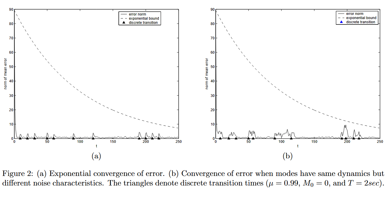
As explained in Section 2, Lemma 2, identical dynamics with different noise characteristics in each discrete state might still make the system observable in the stochastic hybrid context. We demonstrate this by designing an exponentially convergent hybrid estimator for a switched aircraft trajectory - the two discrete states correspond to
2
∘
2^\circ
2∘ per second turns with different process noise covariances. This is shown in Figure (2(b)).
如第 2 节引理 2 所述,在随机混合系统框架下,即使各离散状态的动力学特性相同,只要噪声特性不同,系统仍可能具有可观测性。我们通过为飞行器切换轨迹设计指数收敛的混合估计器来验证这一点——两个离散状态均为
2
∘
/
s
2^\circ/\text{s}
2∘/s 的转弯运动,但过程噪声协方差不同。结果如图 2(b) 所示。
5 Conclusions
5 结论
In this paper, we have extended the definition of observability to include stochastic linear hybrid systems, and have used prior knowledge of system noise characteristics to improve the observability conditions for a discrete-time stochastic linear hybrid system. We have also found bounds on the time between discrete transitions to guarantee the exponential convergence of hybrid estimators for such systems. An interesting direction for future work would be the extension of these results to hybrid systems with continuous state resets.
本文将可观测性定义推广至随机线性混合系统,利用系统噪声特性的先验知识,改进了离散时间随机线性混合系统的可观测性条件。同时,确定了离散切换间隔时间的界,以保证此类系统混合估计器的指数收敛性。未来研究的一个重要方向是,将本文结果推广到含连续状态重置的混合系统中。
References
参考文献
[1] Y. Bar-Shalom and X.R. Li. Estimation and Tracking: Principles, Techniques, and Software. Artech House, Boston, 1993.
Y. Bar-Shalom, X.R. Li. 估计与跟踪:原理、技术及软件[M]. 波士顿:Artech House 出版社, 1993.
[2] T. Kailath. Linear Systems. Prentice Hall, 1980.
T. Kailath. 线性系统[M]. 新泽西:Prentice Hall 出版社, 1980.
[3] P.J. Ramadge. Observability of discrete event-systems. In Proceedings of the 25th IEEE Conference on Decision and Control, pages 1108–1112, Athens, Greece, 1986.
P.J. Ramadge. 离散事件系统的可观测性[C]. 第 25 届 IEEE 决策与控制会议论文集, 希腊雅典, 1986: 1108-1112.
[4] C.M. Özveren and A.S. Willsky. Observability of discrete event dynamic systems. IEEE Transactions on Automatic Control, 35:797–806, 1990.
C.M. Özveren, A.S. Willsky. 离散事件动态系统的可观测性[J]. IEEE 自动控制汇刊, 1990, 35: 797-806.
[5] A. Alessandri and P. Coletta. Design of Luenberger observers for a class of hybrid linear systems. In M. D. DiBenedetto and A. Sangiovanni-Vincentelli, editors, Hybrid Systems: Computation and Control. LNCS, volume 2034, pages 7–18. Springer-Verlag, 2001.
A. Alessandri, P. Coletta. 一类线性混合系统的龙伯格观测器设计[C]. M.D. DiBenedetto, A. Sangiovanni-Vincentelli 主编. 混合系统:计算与控制. LNCS 第 2034 卷. 柏林:Springer-Verlag 出版社, 2001: 7-18.
[6] A. Balluchi, L. Benvenuti, M.D. Di Benedetto, and A.L. Sangiovanni-Vincentelli. Design of observers for hybrid systems. In C. Tomlin and M.R. Greenstreet, editors, Hybrid Systems: Computation and Control. LNCS, volume 2289, pages 76–89. Springer-Verlag, 2002.
A. Balluchi, L. Benvenuti, M.D. Di Benedetto, A.L. Sangiovanni-Vincentelli. 混合系统的观测器设计[C]. C. Tomlin, M.R. Greenstreet 主编. 混合系统:计算与控制. LNCS 第 2289 卷. 柏林:Springer-Verlag 出版社, 2002: 76-89.
[7] A. Bemporad, G. Ferrari, and M. Morari. Observability and controllability of piecewise affine and hybrid systems. IEEE Transactions on Automatic Control, 45(10):1864–1876, 2000.
A. Bemporad, G. Ferrari, M. Morari. 分段仿射系统与混合系统的可观测性和能控性[J]. IEEE 自动控制汇刊, 2000, 45(10): 1864-1876.
[8] R. Vidal, A. Chiuso, S. Soatto, and S. Sastry. Observability of linear hybrid systems. In Hybrid Systems: Computation and Control. LNCS. Springer-Verlag, 2003. submitted.
R. Vidal, A. Chiuso, S. Soatto, S. Sastry. 线性混合系统的可观测性[C]. 混合系统:计算与控制会议论文集. LNCS. 柏林:Springer-Verlag 出版社, 2003(已投稿).
[9] Y. Baram and T. Kailath. Estimability and regulability of linear systems. IEEE Transactions on Automatic Control, 33(12):1116–1121, 1988.
Y. Baram, T. Kailath. 线性系统的可估计性与可调节性[J]. IEEE 自动控制汇刊, 1988, 33(12): 1116-1121.
[10] L.R. Rabiner and B.H. Juang. An introduction to Hidden Markov Models. IEEE Transactions on Acoustics, Speech, and Signal Processing, 3(1):4–16, 1986.
L.R. Rabiner, B.H. Juang. 隐马尔可夫模型导论[J]. IEEE 声学、语音与信号处理汇刊, 1986, 3(1): 4-16.
[11] E.F. Cost and J.B.R. do Val. On the detectability and observability of discrete-time markov jump linear systems. In Proceedings of the 39th IEEE Conference on Decision and Control, Sydney, Australia, December 2000.
E.F. Cost, J.B.R. do Val. 离散时间马尔可夫跳变线性系统的可检测性与可观测性[C]. 第 39 届 IEEE 决策与控制会议论文集, 澳大利亚悉尼, 2000 年 12 月.
[12] R. Vidal, A. Chiuso, and S. Soatto. Observability and identifiability of jump linear systems. In Proceedings of the 41th IEEE Conference on Decision and Control, Las Vegas, NV, December 2002.
R. Vidal, A. Chiuso, S. Soatto. 跳变线性系统的可观测性与可辨识性[C]. 第 41 届 IEEE 决策与控制会议论文集, 美国内华达州拉斯维加斯, 2002 年 12 月.
[13] T. Kailath, A.H. Sayed, and B. Hassibi. Linear Estimation. Prentice Hall, New Jersey, 2000.
T. Kailath, A.H. Sayed, B. Hassibi. 线性估计[M]. 新泽西:Prentice Hall 出版社, 2000.
[14] C. Van Loan. The sensitivity of the matrix exponential. SIAM Journal of Numerical Analysis, 14(6):971–981, December 1977.
C. Van Loan. 矩阵指数的敏感性[J]. SIAM 数值分析杂志, 1977, 14(6): 971-981.
- 随机线性混合系统的可观测性准则与估计器设计(篇 1)-优快云博客
https://blog.youkuaiyun.com/u013669912/article/details/153995165
via:
- Observability Criteria and Estimator Design for Stochastic Linear
Hybrid Systems - ECC03_HBT.pdf
https://www.mit.edu/~hamsa/pubs/ECC03_HBT.pdf


 1万+
1万+

 被折叠的 条评论
为什么被折叠?
被折叠的 条评论
为什么被折叠?
 到【灌水乐园】发言


