以太网最小帧应用在现代网络环境下的演变

注：本文为 “以太网最小帧” 相关文章及 3 篇讨论合辑。

英文引文，机翻未校。
中文引文，未整理。

---

2 Ethernet

2 以太网

We now turn to a deeper analysis of the ubiquitous Ethernet LAN protocol. Current user-level Ethernet today (2013) is usually 100 Mbps, with Gigabit Ethernet standard in server rooms and backbones, but because Ethernet speed scales in odd ways, we will start with the 10 Mbps formulation. While the 10 Mbps speed is obsolete, and while even the Ethernet collision mechanism is largely obsolete, collision management itself continues to play a significant role in wireless networks.
现在，我们转向对无处不在的以太网 LAN 协议的更深入分析。目前（2013 年）的用户级以太网通常为 100 Mbps，服务器机房和骨干网采用千兆以太网标准，但由于以太网速度以奇怪的方式扩展，我们将从 10 Mbps 公式开始。虽然 10 Mbps 的速度已经过时，甚至以太网冲突机制也已基本过时，但冲突管理本身在无线网络中继续发挥着重要作用。

2.1 10-Mbps classic Ethernet

2.1 10 Mbps 经典以太网

The original Ethernet specification was the 1976 paper of Metcalfe and Boggs, [MB76]_. The data rate was 10 megabits per second, and all connections were made with coaxial cable instead of today’s twisted pair. In its original form, an Ethernet was a broadcast bus, which meant that all packets were, at least at the physical level, broadcast onto the shared medium and could be seen, theoretically, by all other nodes. If two nodes transmitted at the same time, there was a collision; proper handling of collisions was an important part of the access-mediation strategy for the shared medium. Data was transmitted using Manchester encoding; see 4.1.3 Manchester_.
最初的以太网规范是 Metcalfe 和 Boggs 在 1976 年的论文 [MB76]。数据速率为每秒 10 Mb，所有连接均使用同轴电缆进行，而不是今天的双绞线。在其原始形式中，以太网是广播总线，这意味着所有数据包至少在物理层面上都广播到共享介质上，理论上所有其他节点都可以看到。如果两个节点同时传输，则发生冲突;正确处理冲突是共享介质的访问中介策略的重要组成部分。数据使用 Manchester 编码传输;见 4.1.3 曼彻斯特。

The linear bus structure could be modified with repeaters (below), into an arbitrary tree structure, though loops remain something of a problem even with today’s Ethernet.
线性总线结构可以用中继器（下图）修改为任意的树形结构，尽管即使在今天的以太网中，循环仍然是一个问题。

Whenever two stations transmitted at the same time, the signals would collide, and interfere with one another; both transmissions would fail as a result. In order to minimize collision loss, each station implemented the following:
每当两个电台同时传输时，信号就会发生碰撞并相互干扰;因此，两种传输都将失败。为了最大限度地减少碰撞损失，每个站点实施了以下措施：

1. Before transmission, wait for the line to become quiet
   传输前，请等待线路安静
2. While transmitting, continually monitor the line for signs that a collision has occurred; if a collision happens, then cease transmitting
   传输时，持续监控线路是否有发生冲突的迹象;如果发生冲突，则停止传输
3. If a collision occurs, use a backoff-and-retransmit strategy
   如果发生冲突，请使用 backoff-and-retransmit 策略

These properties can be summarized with the CSMA/CD acronym: Carrier Sense, Multiple Access, Collision Detect. (The term “carrier sense” was used by Metcalfe and Boggs as a synonym for “signal sense”; there is no literal carrier frequency to be sensed.) It should be emphasized that collisions are a normal event in Ethernet, well-handled by the mechanisms above.
这些特性可以用 CSMA/CD 首字母缩略词来概括：载波侦听、多址访问、冲突检测。（Metcalfe 和 Boggs 将术语“载波感应”用作“信号感应”的同义词;没有要感应的字面载波频率。应该强调的是，冲突是以太网中的正常事件，上述机制可以很好地处理。

Classic Ethernet came in version 1 [1980, DEC-Intel-Xerox], version 2 [1982, DIX], and IEEE 802.3. There are some minor electrical differences between these, and one rather substantial packet-format difference. In addition to these, the Berkeley Unix trailing-headers packet format was used for a while.
传统以太网有版本 1 [1980， DEC-Intel-Xerox]、版本 2 [1982， DIX] 和 IEEE 802.3。这些之间有一些细微的电气差异，还有一个相当大的数据包格式差异。除此之外，Berkeley Unix 尾随标头数据包格式还使用了一段时间。

There were three physical formats for 10 Mbps Ethernet cable: thick coax (10BASE-5), thin coax (10BASE-2), and, last to arrive, twisted pair (10BASE-T). Thick coax was the original; economics drove the successive development of the later two. The cheaper twisted-pair cabling eventually almost entirely displaced coax, at least for host connections.
10 Mbps 以太网电缆有三种物理格式：粗同轴电缆 （10BASE-5）、细同轴电缆 （10BASE-2） 和最后到达的双绞线 （10BASE-T）。粗哄骗是原来的;经济学推动了后两者的连续发展。更便宜的双绞线布线最终几乎完全取代了同轴电缆，至少对于主机连接来说是这样。

The original specification included support for repeaters, which were in effect signal amplifiers although they might attempt to clean up a noisy signal. Repeaters processed each bit individually and did no buffering. In the telecom world, a repeater might be called a digital regenerator. A repeater with more than two ports was commonly called a hub; hubs allowed branching and thus much more complex topologies.
最初的规范包括对中继器的支持，中继器实际上是信号放大器，尽管它们可能会尝试清理嘈杂的信号。中继器单独处理每个位，不进行缓冲。在电信领域，中继器可能被称为数字再生器。具有两个以上端口的中继器通常称为集线器;集线器允许分支，因此拓扑结构要复杂得多。

Bridges – later known as switches – came along a short time later. While repeaters act at the bit layer, a switch reads in and forwards an entire packet as a unit, and the destination address is likely consulted to determine to where the packet is forwarded. Originally, switches were seen as providing interconnection (“bridging”) between separate Ethernets, but later a switched Ethernet was seen as one large “virtual” Ethernet. We return to switching below in 2.4 Ethernet Switches_.
桥梁——后来被称为 switches——不久后出现。当中继器在位层工作时，交换机将整个数据包作为一个单元读入和转发，并且可能会参考目标地址以确定数据包转发到的位置。最初，交换机被视为在单独的以太网之间提供互连（“桥接”），但后来交换以太网被视为一个大型“虚拟”以太网。我们在下面的 2.4 以太网交换机中返回交换。

Hubs propagate collisions; switches do not. If the signal representing a collision were to arrive at one port of a hub, it would, like any other signal, be retransmitted out all other ports. If a switch were to detect a collision one one port, no other ports would be involved; only packets received successfully are ever retransmitted out other ports.
集线器传播碰撞;switches 则不需要。如果表示冲突的信号到达集线器的一个端口，它将像任何其他信号一样，从所有其他端口重新传输出去。如果交换机要检测到一个端口的冲突，则不会涉及其他端口;只有成功接收的数据包才会从其他端口重新传输出去。

In coaxial-cable installations, one long run of coax snaked around the computer room or suite of offices; each computer connected somewhere along the cable. Thin coax allowed the use of T-connectors to attach hosts; connections were made to thick coax via taps, often literally drilled into the coax central conductor. In a standalone installation one run of coax might be the entire Ethernet; otherwise, somewhere a repeater would be attached to allow connection to somewhere else.
在同轴电缆安装中，一根长长的同轴电缆在机房或办公室套件周围蜿蜒而行;每台计算机都沿电缆连接了某个位置。细同轴电缆允许使用 T 型连接器连接主机;通过水龙头连接到粗同轴电缆，通常从字面上钻入同轴电缆中央导体。在独立安装中，一条同轴电缆可能是整个以太网;否则，将在某个位置连接中继器以允许连接到另一个位置。

Twisted-pair does not allow mid-cable attachment; it is only used for point-to-point links between hosts, switches and hubs. In a twisted-pair installation, each cable runs between the computer location and a central wiring closest (generally much more convenient than trying to snake coax all around the building). Originally each cable in the wiring closet plugged into a hub; nowadays the hub has likely been replaced by a switch.
双绞线不允许连接中间电缆;它仅用于主机、交换机和 Hub 之间的点对点链路。在双绞线安装中，每根电缆都位于计算机位置和最近的中央布线之间（通常比试图在建筑物周围蜿蜒诱骗要方便得多）。最初，配线柜中的每根电缆都插入一个集线器;如今，集线器可能已被 Switch 取代。

There is still a role for hubs today when one wants to monitor the Ethernet signal from A to B (eg for intrusion detection analysis), although some switches now also support a form of monitoring.
今天，当人们想要监控从 A 到 B 的以太网信号时（例如用于入侵检测分析），集线器仍然发挥着作用，尽管一些交换机现在也支持某种形式的监控。

All three cable formats could interconnect, although only through repeaters and hubs, and all used the same 10 Mbps transmission speed. While twisted-pair cable is still used by 100 Mbps Ethernet, it generally needs to be a higher-performance version known as Category 5, versus the 10 Mbps Category 3.
所有三种电缆格式都可以互连，但只能通过中继器和集线器，并且都使用相同的 10 Mbps 传输速度。虽然 100 Mbps 以太网仍然使用双绞线电缆，但它通常需要是称为 5 类的更高性能版本，而不是 10 Mbps 3 类。

Here is the format of a typical Ethernet packet (DIX specification):
以下是典型以太网数据包的格式（DIX 规范）：

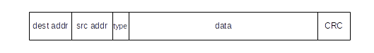
The destination and source addresses are 48-bit quantities; the type is 16 bits, the data length is variable up to a maximum of 1500 bytes, and the final CRC checksum is 32 bits. The checksum is added by the Ethernet hardware, never by the host software. There is also a preamble, not shown: a block of 1 bits followed by a 0, in the front of the packet, for synchronization. The type field identifies the next higher protocol layer; a few common type values are 0x0800 = IP, 0x8137 = IPX, 0x0806 = ARP.
目标地址和源地址为 48 位数量;类型为 16 位，数据长度可变，最大为 1500 字节，最终 CRC 校验和为 32 位。校验和由以太网硬件添加，而不是由主机软件添加。还有一个未显示的前导码：一个 1 位块，后跟一个 0，位于数据包的前面，用于同步。type 字段标识下一个更高的协议层;一些常见的类型值是 0x0800 = IP、0x8137 = IPX 0x0806 = ARP。

The IEEE 802.3 specification replaced the type field by the length field, though this change never caught on. The two formats can be distinguished as long as the type values used are larger than the maximum Ethernet length of 1500 (or 0x05dc); the type values given in the previous paragraph all meet this condition.
IEEE 802.3 规范将 type 字段替换为 length 字段，尽管这一变化从未流行起来。只要使用的类型值大于最大以太网长度 1500（或 0x05dc），就可以区分这两种格式;上一段中给出的 type 值都满足此条件。

Each Ethernet card has a (hopefully unique) physical address in ROM; by default any packet sent to this address will be received by the board and passed up to the host system. Packets addressed to other physical addresses will be seen by the card, but ignored (by default). All Ethernet devices also agree on a broadcast address of all 1’s: a packet sent to the broadcast address will be delivered to all attached hosts.
每个以太网卡在 ROM 中都有一个（希望是唯一的）物理地址;默认情况下，发送到此地址的任何数据包都将被主板接收并向上传递到主机系统。卡将看到寻址到其他物理地址的数据包，但默认情况下会被忽略。所有以太网设备还同意所有 1 的广播地址：发送到广播地址的数据包将被传送到所有连接的主机。

It is sometimes possible to change the physical address of a given card in software. It is almost universally possible to put a given card into promiscuous mode, meaning that all packets on the network, no matter what the destination address, are delivered to the attached host. This mode was originally intended for diagnostic purposes but became best known for the security breach it opens: it was once not unusual to find a host with network board in promiscuous mode and with a process collecting the first 100 bytes (presumably including userid and password) of every telnet connection.
有时可以在软件中更改给定卡的物理地址。几乎普遍可以将给定卡置于混杂模式，这意味着网络上的所有数据包，无论目标地址是什么，都会传送到连接的主机。这种模式最初用于诊断目的，但因其打开的安全漏洞而广为人知：曾经发现网络板处于混杂模式的主机，并且进程收集每个 telnet 连接的前 100 个字节（可能包括用户 ID 和密码）并不罕见。

2.1.1 Ethernet Multicast

2.1.1 以太网组播

Another category of Ethernet addresses is multicast, used to transmit to a set of stations; streaming video to multiple simultaneous viewers might use Ethernet multicast. The lowest-order bit in the first byte of an address indicates whether the address is physical or multicast. To receive packets addressed to a given multicast address, the host must inform its network interface that it wishes to do so; once this is done, any arriving packets addressed to that multicast address are forwarded to the host. The set of subscribers to a given multicast address may be called a multicast group. While higher-level protocols might prefer that the subscribing host also notifies some other host, eg the sender, this is not required, although that might be the easiest way to learn the multicast address involved. If several hosts subscribe to the same multicast address, then each will receive a copy of each multicast packet transmitted.
另一类以太网地址是多播，用于传输到一组工作站;将视频流式传输到多个同时观看者可能会使用以太网多播。地址第一个字节中的最低顺序位指示地址是物理地址还是多播地址。要接收寻址到给定多播地址的数据包，主机必须通知其网络接口它希望这样做;完成此作后，发送到该组播地址的任何到达数据包都将转发到主机。给定组播地址的订阅者集可称为组播组。虽然更高级别的协议可能更希望订阅主机也通知其他主机，例如发送者，但这不是必需的，尽管这可能是了解所涉及的多播地址的最简单方法。如果多个主机订阅相同的多播地址，则每个主机都将收到传输的每个多播数据包的副本。

If switches (below) are involved, they must normally forward multicast packets on all outbound links, exactly as they do for broadcast packets; switches have no obvious way of telling where multicast subscribers might be. To avoid this, some switches do try to engage in some form of multicast filtering, sometimes by snooping on higher-layer multicast protocols. Multicast Ethernet is seldom used by IPv4, but plays a larger role in IPv6 configuration.
如果涉及交换机（如下），则它们通常必须在所有出站链路上转发多播数据包，就像它们对广播数据包所做的那样;交换机无法明显地判断多播订阅者可能在哪里。为避免这种情况，一些交换机确实会尝试进行某种形式的组播过滤，有时通过窥探更高层的组播协议。多播以太网很少被 IPv4 使用，但在 IPv6 配置中起着更大的作用。

The second-to-lowest-order bit of the Ethernet address indicates, in the case of physical addresses, whether the address is believed to be globally unique or if it is only locally unique; this is known as the Universal/Local bit. When (global) Ethernet IDs are assigned by the manufacturer, the first three bytes serve to indicate the manufacturer. As long as the manufacturer involved is diligent in assigning the second three bytes, every manufacturer-provided Ethernet address should be globally unique. Lapses, however, are not unheard of.
以太网地址的二阶到最低位表示，对于物理地址，该地址是被认为是全局唯一的，还是仅在本地唯一;这称为 Universal/Local 位。当制造商分配（全局）以太网 ID 时，前三个字节用于指示制造商。只要所涉及的制造商认真分配后三个字节，制造商提供的每个以太网地址都应该是全局唯一的。然而，失误并非闻所未闻。

2.1.2 The Slot Time and Collisions

2.1.2 插槽时间和碰撞

The diameter of an Ethernet is the maximum distance between any pair of stations. The actual total length of cable can be much greater than this, if, for example, the topology is a “star” configuration. The maximum allowed diameter, measured in bits, is limited to 232 (a sample “budget” for this is below). This makes the round-trip-time 464 bits. As each station involved in a collision discovers it, it transmits a special jam signal of up to 48 bits. These 48 jam bits bring the total above to 512 bits, or 64 bytes. The time to send these 512 bits is the slot time of an Ethernet; time intervals on Ethernet are often described in bit times but in conventional time units the slot time is 51.2 µsec.
以太网的直径是任何一对工作站之间的最大距离。电缆的实际总长度可能远大于此长度，例如，如果拓扑是 “星形” 配置。允许的最大直径（以位为单位）限制为 232（示例“预算”如下）。这使得往返时间为 464 位。当涉及碰撞的每个站点发现它时，它会传输一个高达 48 位的特殊干扰信号。这 48 个 jam 位使上述总数达到 512 位，即 64 字节。发送这 512 位的时间是以太网的时隙时间;以太网上的时间间隔通常以位时间描述，但在传统时间单位中，时隙时间为 51.2 μsec。

The value of the slot time determines several subsequent aspects of Ethernet. If a station has transmitted for one slot time, then no collision can occur (unless there is a hardware error) for the remainder of that packet. This is because one slot time is enough time for any other station to have realized that the first station has started transmitting, so after that time they will wait for the first station to finish. Thus, after one slot time a station is said to have acquired the network. The slot time is also used as the basic interval for retransmission scheduling, below.
slot time 的值决定了 Ethernet 的几个后续方面。如果一个工作站已经传输了一个时隙时间，则该数据包的其余部分不会发生冲突（除非存在硬件错误）。这是因为一个时隙时间足以让任何其他电台意识到第一个电台已经开始传输，因此在此之后，他们将等待第一个电台完成。因此，在一个时隙时间之后，可以说一个电台已经获得了该网络。slot 时间也用作 retransmission scheduling 的基本间隔，如下所示。

Conversely, a collision can be received, in principle, at any point up until the end of the slot time. As a result, Ethernet has a minimum packet size, equal to the slot time, ie 64 bytes (or 46 bytes in the data portion). A station transmitting a packet this size is assured that if a collision were to occur, the sender would detect it (and be able to apply the retransmission algorithm, below). Smaller packets might collide and yet the sender not know it, ultimately leading to greatly reduced throughput.
相反，原则上，在 slot 时间结束之前的任何时间点都可以接收 collision。因此，以太网具有最小数据包大小，等于插槽时间，即 64 字节（或数据部分的 46 字节）。可以确保传输这种大小的数据包的站点在发生冲突时，发送方会检测到它（并能够应用下面的重传算法）。较小的数据包可能会发生冲突，但发送方并不知道，最终导致吞吐量大大降低。

If we need to send less than 46 bytes of data (for example, a 40-byte TCP ACK packet), the Ethernet packet must be padded out to the minimum length. As a result, all protocols running on top of Ethernet need to provide some way to specify the actual data length, as it cannot be inferred from the received packet size.
如果我们需要发送少于 46 字节的数据（例如，一个 40 字节的 TCP ACK 数据包），则必须将以太网数据包填充到最小长度。因此，在 Ethernet 上运行的所有协议都需要提供某种方法来指定实际数据长度，因为它无法从接收到的数据包大小推断出来。

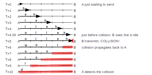
As a specific example of a collision occurring as late as possible, consider the diagram below. A and B are 5 units apart, and the bandwidth is 1 byte/unit. A begins sending “helloworld” at T=0; B starts sending just as A’s message arrives, at T=5. B has listened before transmitting, but A’s signal was not yet evident. A doesn’t discover the collision until 10 units have elapsed, which is twice the distance.
作为冲突发生得越晚的具体示例，请考虑下图。A 和 B 相距 5 个单位，带宽为 1 字节/单位。A 在 T=0 时开始发送 “helloworld”;B 在 A 的消息到达时开始发送，T=5。B 在传输之前已经监听了，但 A 的信号还不明显。A 在经过 10 个单位后才发现碰撞，这是距离的两倍。

Here are typical maximum values for the delay in 10 Mbps Ethernet due to various components. These are taken from the Digital-Intel-Xerox (DIX) standard of 1982, except that “point-to-point link cable” is replaced by standard cable. The DIX specification allows 1500m of coax with two repeaters and 1000m of point-to-point cable; the table below shows 2500m of coax and four repeaters, following the later IEEE 802.3 Ethernet specification. Some of the more obscure delays have been eliminated. Entries are one-way delay times, in bits. The maximum path may have four repeaters, and ten transceivers (simple electronic devices between the coax cable and the NI cards), each with its drop cable (two transceivers per repeater, plus one at each endpoint).
以下是由于各种组件而导致的 10 Mbps 以太网延迟的典型最大值。这些取自 1982 年的 Digital-Intel-Xerox （DIX） 标准，只是“点对点链路电缆”被标准电缆取代。DIX 规格允许 1500m 的同轴电缆，带有两个中继器和 1000m 的点对点电缆;下表显示了 2500m 的同轴电缆和四个中继器，遵循后来的 IEEE 802.3 以太网规范。一些更模糊的延迟已被消除。条目是单向延迟时间（以位为单位）。最大路径可以有四个中继器和十个收发器（同轴电缆和 NI 卡之间的简单电子设备），每个收发器都有自己的引入电缆（每个中继器两个收发器，每个端点一个）。

Ethernet delay budget
以太网延迟预算

item	length	delay, in bits	explanation (c = speed of light)
coax	2500M	110 bits	23 meters/bit (.77c)
transceiver cables	500M	25 bits	19.5 meters/bit (.65c)
transceivers		40 bits, max 10 units	4 bits each
repeaters		25 bits, max 4 units	6+ bits each (DIX 7.6.4.1)
encoders		20 bits, max 10 units	2 bits each (for signal generation)

The total here is 220 bits; in a full accounting it would be 232. Some of the numbers shown are a little high, but there are also signal rise time delays, sense delays, and timer delays that have been omitted. It works out fairly closely.
这里的总数是 220 位;在完整的会计核算中，它将是 232。显示的一些数字有点高，但也有被省略的信号上升时间延迟、检测延迟和定时器延迟。它的效果相当接近。

Implicit in the delay budget table above is the “length” of a bit. The speed of propagation in copper is about 0.77×c, where c=3×108 m/sec = 300 m/µsec is the speed of light in vacuum. So, in 0.1 microseconds (the time to send one bit at 10 Mbps), the signal propagates approximately 0.77×c×10-7 = 23 meters.
上面的 delay budget 表中隐含的是 bit 的 “length” 。铜中的传播速度约为 0.77×c，其中 c=3×108 m/sec = 300 m/μsec 是真空中的光速。因此，在 0.1 微秒（以 10 Mbps 发送一位的时间）中，信号传播的距离约为 0.77×c×10-7 = 23 米。

Ethernet packets also have a maximum packet size, of 1500 bytes. This limit is primarily for the sake of fairness, so one station cannot unduly monopolize the cable (and also so stations can reserve buffers guaranteed to hold an entire packet). At one time hardware vendors often marketed their own incompatible “extensions” to Ethernet which enlarged the maximum packet size to as much as 4KB. There is no technical reason, actually, not to do this, except compatibility.
以太网数据包的最大数据包大小为 1500 字节。这个限制主要是为了公平起见，所以一个站不能过度垄断电缆（也为了让站可以保留保证容纳整个数据包的缓冲区）。曾经有一段时间，硬件供应商经常推销他们自己不兼容的以太网“扩展”，这将最大数据包大小扩大到 4KB。实际上，除了兼容性之外，没有技术理由不这样做。

The signal loss in any single segment of cable is limited to 8.5 db, or about 14% of original strength. Repeaters will restore the signal to its original strength. The reason for the per-segment length restriction is that Ethernet collision detection requires a strict limit on how much the remote signal can be allowed to lose strength. It is possible for a station to detect and reliably read very weak remote signals, but not at the same time that it is transmitting locally. This is exactly what must be done, though, for collision detection to work: remote signals must arrive with sufficient strength to be heard even while the receiving station is itself transmitting. The per-segment limit, then, has nothing to do with the overall length limit; the latter is set only to ensure that a sender is guaranteed of detecting a collision, even if it sends the minimum-sized packet.
任何单段电缆的信号损失都限制为 8.5 分贝，或原始强度的 14% 左右。中继器会将信号恢复到其原始强度。每个分段长度限制的原因是，以太网冲突检测要求严格限制允许远程信号失去强度的程度。电台可以检测并可靠地读取非常微弱的远程信号，但不能在本地传输的同时读取。然而，这正是要使碰撞检测工作所必须做的事情：远程信号必须具有足够的强度，即使在接收站本身正在传输时也能被听到。因此，每个段的限制与总长度限制无关;设置后者只是为了确保保证发送方检测到冲突，即使它发送最小大小的数据包也是如此。

2.1.3 Exponential Backoff Algorithm

2.1.3 指数退避算法

Whenever there is a collision the exponential backoff algorithm is used to determine when each station will retry its transmission. Backoff here is called exponential because the range from which the backoff value is chosen is doubled after every successive collision involving the same packet. Here is the full Ethernet transmission algorithm, including backoff and retransmissions:
每当发生冲突时，指数回退算法用于确定每个站点何时重试其传输。此处的回退称为指数，因为在涉及同一数据包的每次连续冲突后，选择回退值的范围都会加倍。以下是完整的以太网传输算法，包括回退和重传：

1. Listen before transmitting (“carrier detect”)
   传输前监听 （“carrier detect”）
2. If line is busy, wait for sender to stop and then wait an additional 9.6 microseconds (96 bits). One consequence of this is that there is always a 96-bit gap between packets, so packets do not run together.
   如果线路繁忙，请等待发送方停止，然后再等待 9.6 微秒（96 位）。这样做的一个结果是，数据包之间始终存在 96 位的间隙，因此数据包不会一起运行。
3. Transmit while simultaneously monitoring for collisions
   传输，同时监控冲突
4. If a collision does occur, send the jam signal, and choose a backoff time as follows: For transmission N, 1≤N≤10 (N=0 represents the original attempt), choose k randomly with 0 ≤ k < 2N. Wait k slot times (k×51.2 µsec). Then check if the line is idle, waiting if necessary for someone else to finish, and then retry step 3. For 11≤N≤15, choose k randomly with 0 ≤ k < 1024 (= 210)
   如果确实发生冲突，则发送干扰信号，并按如下方式选择回退时间：对于传输 N，1≤N≤10（N=0 表示原始尝试），随机选择 k，其中 0 ≤ k < 2N。等待 k 个时隙时间 （k×51.2 μsec）。然后检查线路是否处于空闲状态，如有必要，请等待其他人完成，然后重试步骤 3。对于 11≤N≤15，随机选择 k，其中 0 ≤ k < 1024 （= 210）
5. If we reach N=16 (16 transmission attempts), give up.
   如果我们达到 N=16（16 次传输尝试），就放弃。

If an Ethernet sender does not reach step 5, there is a very high probability that the packet was delivered successfully.
如果以太网发送方未到达步骤 5，则数据包成功传送的可能性非常高。

Exponential backoff means that if two hosts have waited for a third to finish and transmit simultaneously, and collide, then when N=1 they have a 50% chance of recollision; when N=2 there is a 25% chance, etc. When N≥10 the maximum wait is 52 milliseconds; without this cutoff the maximum wait at N=15 would be 1.5 seconds. As indicated above in the minimum-packet-size discussion, this retransmission strategy assumes that the sender is able to detect the collision while it is still sending, so it knows that the packet must be resent.
指数回退意味着，如果两个主机等待第三个主机完成并同时传输并发生碰撞，那么当 N=1 时，它们有 50% 的几率再次冲突;当 N=2 时，有 25% 的几率，依此类推。当 N≥10 时，最大等待时间为 52 毫秒;如果没有此截止时间，N=15 时的最大等待时间为 1.5 秒。如上文 minimum-packet-size 讨论中所示，此重传策略假定发送方能够在仍在发送时检测到冲突，因此它知道必须重新发送数据包。

In the following diagram is an example of several stations attempting to transmit all at once, and using the above transmission/backoff algorithm to sort out who actually gets to acquire the channel. We assume we have five prospective senders A1, A2, A3, A4 and A5, all waiting for a sixth station to finish. We will assume that collision detection always takes one slot time (it will take much less for nodes closer together) and that the slot start-times for each station are synchronized; this allows us to measure time in slots. A solid arrow at the start of a slot means that sender began transmission in that slot; a red X signifies a collision. If a collision occurs, the backoff value k is shown underneath. A dashed line shows the station waiting k slots for its next attempt.
下图中是一个示例，其中多个站点尝试一次传输所有通道，并使用上述传输/回退算法来分辨谁实际可以获取通道。我们假设我们有 5 个潜在发送者 A1、A2、A3、A4 和 A5，都在等待第六个站点完成。我们假设碰撞检测总是需要一个 slot 时间（节点靠得更近时，花费的时间会少得多），并且每个 station 的 slot 开始时间是同步的;这允许我们测量 slot 中的时间。时隙开头的实心箭头表示发送方在该时隙中开始传输;红色 X 表示碰撞。如果发生冲突，则 backoff 值 k 显示在下方。虚线表示等待 k 个插槽进行下一次尝试的工作站。

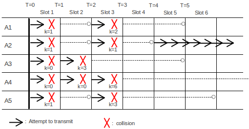
At T=0 we assume the transmitting station finishes, and all the Ai transmit and collide. At T=1, then, each of the Ai has discovered the collision; each chooses a random k<2. Let us assume that A1 chooses k=1, A2 chooses k=1, A3 chooses k=0, A4 chooses k=0, and A5 chooses k=1.
在 T=0 时，我们假设发射站结束，所有 Ai 发射并碰撞。那么，在 T=1 时，每个 Ai 都发现了碰撞;每个 K<2 随机选择一个。假设 A1 中选择 k=1，A2 中选择 k=1，A3 中选择 k=0，A4 中选择 k=0，A5 中选择 k=1。

Those stations choosing k=0 will retransmit immediately, at T=1. This means A3 and A4 collide again, and at T=2 they now choose random k<4. We will Assume A3 chooses k=3 and A4 chooses k=0; A3 will try again at T=2+3=5 while A4 will try again at T=2, that is, now.
那些选择 k=0 的台站将在 T=1 处立即重传。这意味着 A3 和 A4 再次碰撞，在 T=2 时，他们现在选择随机 k<4。假设 A3 中选择 k=3，A4 中选择 k=0;A3 中将在 T=2+3=5 时重试，而 A4 将在 T=2 时重试，即现在。

At T=2, we now have the original A1, A2, and A5 transmitting for the second time, while A4 trying again for the third time. They collide. Let us suppose A1 chooses k=2, A2 chooses k=1, A5 chooses k=3, and A4 chooses k=6 (A4 is choosing k<8 at random). Their scheduled transmission attempt times are now A1 at T=3+2=5, A2 at T=4, A5 at T=6, and A4 at T=9.
在 T=2 时，我们现在有原始的 A1、A2 和 A5 第二次发射，而 A4 第三次再次尝试。他们相撞。假设 A1 中选择 k=2，A2 选择 k=1，A5 选择 k=3，A4 选择 k=6（A4 随机选择 k<8）。他们的计划传输尝试时间现在是 T=3+2=5 时的 A1、T=4 时的 A2、T=6 时的 A5 和 T=9 时的 A4。

At T=3, nobody attempts to transmit. But at T=4, A2 is the only station to transmit, and so successfully seizes the channel. By the time T=5 rolls around, A1 and A3 will check the channel, that is, listen first, and wait for A2 to finish. At T=9, A4 will check the channel again, and also begin waiting for A2 to finish.
在 T=3 时，没有人尝试传输。但在 T=4 时，A2 是唯一发射的电台，因此成功地夺取了频道。当 T=5 滚动时，A1 和 A3 会检查频道，即先监听，然后等待 A2 结束。在 T=9 时，A4 中将再次检查通道，并开始等待 A2 结束。

A maximum of 1024 hosts is allowed on an Ethernet. This number apparently comes from the maximum range for the backoff time as 0 ≤ k < 1024. If there are 1024 hosts simultaneously trying to send, then, once the backoff range has reached k<1024 (N=10), we have a good chance that one station will succeed in seizing the channel, that is; the minimum value of all the random k’s chosen will be unique.
以太网上最多允许 1024 台主机。这个数字显然来自回退时间的最大范围，即 0 ≤ k < 1024。如果有 1024 个主机同时尝试发送，那么，一旦回退范围达到 k<1024 （N=10），我们很有可能一个 station 成功夺取信道，即;所有选择的随机 K 的最小值都是唯一的。

This backoff algorithm is not “fair”, in the sense that the longer a station has been waiting to send, the lower its priority sinks. Newly transmitting stations with N=0 need not delay at all. The Ethernet capture effect, below, illustrates this unfairness.
这种回退算法并不“公平”，因为 station 等待发送的时间越长，其优先级下降就越低。N=0 的新发射台站根本不需要延迟。下面的以太网捕获效果说明了这种不公平。

2.1.4 Capture effect

2.1.4 捕获效果

The capture effect is a scenario illustrating the potential lack of fairness in the exponential backoff algorithm. The unswitched Ethernet must be fully busy, in that each of two senders always has a packet ready to transmit.
捕获效果是一个场景，说明了指数回退算法中可能缺乏公平性。非交换以太网必须完全忙，因为两个发送方中的每一个都有一个数据包可供传输。

Let A and B be two such busy nodes, simultaneously starting to transmit their first packets. They collide. Suppose A wins, and sends. When A is finished, B tries to transmit again. But A has a second packet, and so A tries too. A chooses a backoff k<2 (that is, between 0 and 1 inclusive), but since B is on its second attempt it must choose k<4. This means A is favored to win. Suppose it does.
假设 A 和 B 是两个这样的繁忙节点，同时开始传输它们的第一个数据包。他们相撞。假设 A 获胜，并发送。当 A 完成后，B 尝试再次传输。但是 A 有第二个数据包，所以 A 也尝试了。A 选择回退 k<2（即介于 0 和 1 之间，包括 0 和 1），但由于 B 正在进行第二次尝试，因此它必须选择 k<4。这意味着 A 被看好获胜。假设是这样。

After that transmission is finished, A and B try yet again: A on its first attempt for its third packet, and B on its third attempt for its first packet. Now A again chooses k<2 but B must choose k<8; this time A is much more likely to win. Each time B fails to win a given backoff, its probability of winning the next one is reduced by about 1/2. It is quite possible, and does occur in practice, for B to lose all the backoffs until it reaches the maximum of N=16 attempts; once it has lost the first three or four this is in fact quite likely. At this point B simply discards the packet and goes on to the next one with N reset to 1 and k chosen from {0,1}.
传输完成后，A 和 B 再次尝试：A 第一次尝试其第三个数据包，B 第三次尝试其第一个数据包。现在 A 再次选择 k<2，但 B 必须选择 k<8;这次 A 获胜的可能性要大得多。每次 B 未能赢得给定的 backoff 时，它赢得下一个 backoff 的概率就会降低约 1/2。B 很有可能（并且在实践中确实会发生）丢失所有回退，直到达到 N=16 次尝试的最大值;一旦它失去了前三或四名，这实际上是很有可能的。此时，B 简单地丢弃数据包并继续下一个数据包，N 重置为 1，k 从 {0,1} 中选择。

The capture effect can be fixed with appropriate modification of the backoff algorithm; the Binary Logarithmic Arbitration Method (BLAM) was proposed in [MM94]_. The BLAM algorithm was considered for the then-nascent 100 Mbps “Fast” Ethernet standard. But in the end a hardware strategy won out: Fast Ethernet supports “full-duplex” mode which is collision-free (see 2.2 100 Mbps (Fast) Ethernet_, below). While full-duplex mode is not required for using Fast Ethernet, it was assumed that any sites concerned enough about performance to be worried about the capture effect would opt for full-duplex.
可以通过对 backoff 算法进行适当修改来修复捕获效果;二进制对数仲裁方法 （BLAM） 是在 [MM94] 中提出的。当时新兴的 100 Mbps“快速”以太网标准考虑了 BLAM 算法。但最终硬件策略胜出：快速以太网支持无冲突的“全双工”模式（参见下面的 2.2 100 Mbps（快速）以太网）。虽然使用快速以太网不需要全双工模式，但假设任何足够关心性能而担心捕获效果的站点都会选择全双工。

2.1.5 Hubs and topology

2.1.5 Hub 和拓扑

Ethernet hubs (multiport repeaters) change the topology, but not the fundamental constraints. Hubs allow much more branching; typically, each station in the office now has its own link to the wiring closet. Loops are still forbidden. Before inexpensive switches were widely available, 10BASE-T (twisted pair Ethernet) used hubs heavily; with twisted pair, a device can only connect to the endpoint of the wire. Thus, typically, each host is connected directly to a hub. The maximum diameter of an Ethernet consisting of multiple segments, joined by hubs, is constrained by the round-trip-time, and the need to detect collisions before the sender has completed sending, as before. However, twisted-pair links are required to be much shorter, about 100 meters.
以太网集线器（多端口中继器）会改变拓扑结构，但不会改变基本约束。Hub 允许更多的分支;通常，办公室中的每个工作站现在都有自己的连接点。Loop 仍然被禁止。在廉价交换机广泛使用之前，10BASE-T（双绞线以太网）大量使用集线器;使用双绞线时，设备只能连接到导线的端点。因此，通常，每个主机都直接连接到一个集线器。由多个分段组成的以太网的最大直径（由集线器连接）受往返时间的限制，并且需要像以前一样在发送方完成发送之前检测冲突。但是，双绞线链路需要短得多，大约 100 米。

2.1.6 Errors

2.1.6 错误

Packets can have bits flipped or garbled by electrical noise on the cable; estimates of the frequency with which this occurs range from 1 in 104 to 1 in 106. Bit errors are not uniformly likely; when they occur, they are likely to occur in bursts. Packets can also be lost in hubs, although this appears less likely. Packets can be lost due to collisions only if the sending host makes 16 unsuccessful transmission attempts and gives up. Ethernet packets contain a 32-bit CRC error-detecting code (see 5.4.1 Cyclical Redundancy Check: CRC_) to detect bit errors. Packets can also be misaddressed by the sending host, or, most likely of all, they can arrive at the receiving host at a point when the receiver has no free buffers and thus be dropped by a higher-layer protocol.
数据包的位可能会因电缆上的电噪声而翻转或乱码;这种情况发生的频率估计为 1/104 到 1/106。位错误的可能性并不相同;当它们发生时，它们可能会突然发生。数据包也可能在 Hub 中丢失，尽管这似乎不太可能。只有当发送主机进行了 16 次不成功的传输尝试并放弃时，数据包才会因冲突而丢失。以太网数据包包含一个 32 位 CRC 错误检测代码（请参阅 5.4.1 循环冗余校验：CRC）来检测位错误。数据包也可能被发送主机错误寻址，或者，它们很可能在接收方没有空闲缓冲区时到达接收主机，从而被更高层的协议丢弃。

2.1.7 CSMA persistence

2.1.7 CSMA 持久性

A carrier-sense/multiple-access transmission strategy is said to be nonpersistent if, when the line is busy, the sender waits a randomly selected time. A strategy is p-persistent if, after waiting for the line to clear, the sender sends with probability p≤1. Ethernet uses 1-persistence. A consequence of 1-persistence is that, if more than one station is waiting for line to clear, then when the line does clear a collision is certain. However, Ethernet then gracefully handles the resulting collision via the usual exponential backoff. If N stations are waiting to transmit, the time required for one station to win the backoff is linear in N.
如果线路繁忙时，发送方等待随机选择的时间，则称载波侦听/多路访问传输策略为非持久性。如果在等待线路清除后，发送方以概率 p≤1 发送，则策略是 p 持久性的。以太网使用 1-persistence。1 持续性的结果是，如果多个站点正在等待线路清理，那么当线路清理时，肯定会发生冲突。但是，以太网随后通过通常的指数回退正常处理生成的冲突。如果 N 个站点正在等待传输，则一个站点赢得回退所需的时间在 N 中是线性的。

When we consider the Wi-Fi collision-handling mechanisms in 3.3 Wi-Fi_, we will see that collisions cannot be handled quite as cheaply: for one thing, there is no way to detect a collision in progress, so the entire packet-transmission time is wasted. In the Wi-Fi case, p-persistence is used with p<1.
当我们考虑 3.3 Wi-Fi 中的 Wi-Fi 冲突处理机制时，我们会发现冲突的处理成本并不高：一方面，无法检测正在进行的冲突，因此整个数据包传输时间都被浪费了。在 Wi-Fi 情况下，p-persistence 与 p<1 一起使用。

An Ethernet broadcast storm was said to occur when there were too many transmission attempts, and most of the available bandwidth was tied up in collisions. A properly functioning classic Ethernet had an effective bandwidth of as much as 50-80% of the nominal 10Mbps capacity, but attempts to transmit more than this typically resulted in successfully transmitting a good deal less.
据说，当传输尝试次数过多时，就会发生以太网广播风暴，并且大部分可用带宽都被冲突所占用。正常运行的传统以太网的有效带宽高达标称 10Mbps 容量的 50-80%，但尝试传输超过此容量通常会导致成功传输的带宽少得多。

2.1.8 Analysis of Classic Ethernet

2.1.8 经典以太网分析

How much time does Ethernet “waste” on collisions? A paradoxical attribute of Ethernet is that raising the transmission-attempt rate on a busy segment can reduce the actual throughput. More transmission attempts can lead to longer contention intervals between packets, as senders use the transmission backoff algorithm to attempt to acquire the channel. What effective throughput can be achieved?
以太网在冲突上“浪费”了多少时间？以太网的一个矛盾属性是，提高繁忙网段上的传输尝试速率会降低实际吞吐量。更多的传输尝试可能会导致数据包之间的争用间隔更长，因为发送方使用传输回退算法来尝试获取通道。可以实现什么有效吞吐量？

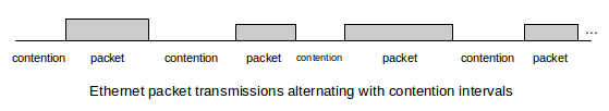
It is convenient to refer to the time between packet transmissions as the contention interval even if there is no actual contention, even if the network is idle. Thus, a timeline for Ethernet always consists of alternating packet transmissions and contention intervals:
即使没有实际的争用，即使网络处于空闲状态，也可以方便地将数据包传输之间的时间称为争用间隔。因此，以太网的时间轴始终由交替的数据包传输和争用间隔组成：

As a first look at contention intervals, assume that there are N stations waiting to transmit at the start of the interval. It turns out that, if all follow the exponential backoff algorithm, we can expect O(N) slot times before one station successfully acquires the channel; thus, Ethernets are happiest when N is small and there are only a few stations simultaneously transmitting. However, multiple stations are not necessarily a severe problem. Often the number of slot times needed turns out to be about N/2, and slot times are short. If N=20, then N/2 is 10 slot times, or 640 bytes. However, one packet time might be 1500 bytes. If packet intervals are 1500 bytes and contention intervals are 640 byes, this gives an overall throughput of 1500/(640+1500) = 70% of capacity. In practice, this seems to be a reasonable upper limit for the throughput of classic shared-media Ethernet.
首先查看争用间隔，假设在间隔开始时有 N 个站点等待传输。事实证明，如果所有站点都遵循指数回退算法，我们可以预期在一个站点成功获取信道之前有 O（N） 个时隙时间;因此，当 N 较小且只有几个站点同时传输时，以太网最受欢迎。但是，多个站点不一定是一个严重的问题。通常所需的插槽时间约为 N/2，而且插槽时间很短。如果 N=20，则 N/2 是 10 个槽时间，即 640 字节。但是，一个数据包时间可能是 1500 字节。如果数据包间隔为 1500 字节，争用间隔为 640 字节，则总吞吐量为 1500/（640+1500） = 容量的 70%。在实践中，这似乎是传统共享媒体以太网吞吐量的合理上限。

2.1.8.1 The ALOHA models

2.1.8.1 ALOHA 模型

We get very similar throughput values when we analyze the Ethernet contention interval using the ALOHA model that was a precursor to Ethernet, and assume a very large number of active senders, each transmitting at a very low rate.
当我们使用 ALOHA 模型（作为以太网的前身）分析以太网争用间隔时，我们得到了非常相似的吞吐量值，并假设有非常多的活动发送方，每个发送方都以非常低的速率传输。

In the ALOHA model, stations transmit packets without listening first for a quiet line or monitoring the transmission for collisions (this models the situation of several ground stations transmitting to a satellite; the ground stations are presumed unable to see one another). To model the success rate of ALOHA, assume all the packets are the same size and let T be the time to send one (fixed-size) packet; T represents the Aloha slot time. We will find the transmission rate that optimizes throughput.
在 ALOHA 模型中，站点在不先侦听静线或监控传输冲突的情况下传输数据包（这模拟了多个地面站向卫星传输的情况;假定地面站无法看到彼此）。为了对 ALOHA 的成功率进行建模，假设所有数据包的大小相同，并设 T 为发送一个（固定大小）数据包的时间;T 代表 Aloha 插槽时间。我们将找到优化吞吐量的传输速率。

The core assumption of this model is that that a large number N of hosts are transmitting, each at a relatively low rate of s packets/slot. Denote by G the average number of transmission attempts per slot; we then have G = Ns. We will derive an expression for S, the average rate of successful transmissions per slot, in terms of G.
此模型的核心假设是，大量 N 台主机正在传输，每台主机的 s 数据包/插槽速率相对较低。用 G 表示每个时隙的平均传输尝试次数;然后我们有 G = Ns。我们将推导出 S 的表达式，即每个时隙的平均成功传输率，以 G 表示。

If two packets overlap during transmissions, both are lost. Thus, a successful transmission requires everyone else quiet for an interval of 2T: if a sender succeeds in the interval from t to t+T, then no other node can have tried to begin transmission in the interval t−T to t+T. The probability of one station transmitting during an interval of time T is G = Ns; the probability of the remaining N−1 stations all quiet for an interval of 2T is (1−s)2(N−1). The probability of a successful transmission is thus
如果两个数据包在传输过程中重叠，则两个数据包都会丢失。因此，成功的传输需要其他人安静 2T 的间隔：如果发送方在从 t 到 t+T 的间隔内成功，则没有其他节点可以尝试在间隔 t−T 到 t+T 内开始传输。在时间间隔 T 内，一个台站发射的概率为 G = Ns;其余 N-1 个台站在 2T 间隔内全部安静的概率为 （1−s）2（N−1）。因此，传输成功的概率为

S = Ns*(1−s)2(N−1)

= G(1−G/N)2N

⟶ Ge-2G as N⟶∞.
 
S = Ns*（1−s）2（N−1） = G（1−G/N）2N ⟶ Ge-2G 为 N⟶∞。

The function S = G e-2G has a maximum at G=1/2, S=1/2e. The rate G=1/2 means that, on average, a transmission is attempted every other slot; this yields the maximum successful-transmission throughput of 1/2e. In other words, at this maximum attempt rate G=1/2, we expect about 2e−1 slot times worth of contention between successful transmissions. What happens to the remaining G−S unsuccessful attempts is not addressed by this model; presumably some higher-level mechanism (eg backoff) leads to retransmissions.
函数 S = G e-2G 在 G=1/2、S=1/2e 时具有最大值。速率 G=1/2 意味着，平均而言，每隔一个时隙尝试一次传输;这产生了 1/2e 的最大成功传输吞吐量。换句话说，在这个最大尝试率 G=1/2 下，我们预计成功传输之间的争用约为 2e−1 时隙时间。该模型没有解决剩余的 G-S 不成功尝试会发生什么;据推测，一些更高级别的机制（例如 backoff）会导致重传。

A given throughput S<1/2e may be achieved at either of two values for G; that is, a given success rate may be due to a comparable attempt rate or else due to a very high attempt rate with a similarly high failure rate.
给定的吞吐量 S<1/2e 可以在 G 的两个值中的任何一个下实现;也就是说，给定的成功率可能是由于可比的尝试率，或者是由于非常高的尝试率和同样高的失败率。

2.1.8.2 ALOHA and Ethernet

2.1.8.2 ALOHA 和以太网

The relevance of the Aloha model to Ethernet is that during one Ethernet slot time there is no way to detect collisions (they haven’t reached the sender yet!) and so the Ethernet contention phase resembles ALOHA with an Aloha slot time T of 51.2 microseconds. Once an Ethernet sender succeeds, however, it continues with a full packet transmission, which is presumably many times longer than T.
Aloha 模型与以太网的相关性在于，在一个以太网时隙时间内，无法检测冲突（它们尚未到达发送方），因此以太网争用阶段类似于 ALOHA，Aloha 时隙时间 T 为 51.2 微秒。但是，一旦以太网发送方成功，它就会继续进行完整的数据包传输，这可能比 T 长很多倍。

The average length of the contention interval, at the maximum throughput calculated above, is 2e−1 slot times (from ALOHA); recall that our model here supposed many senders sending at very low individual rates. This is the minimum contention interval; with lower loads the contention interval is longer due to greater idle times and with higher loads the contention interval is longer due to more collisions.
在上面计算的最大吞吐量下，争用间隔的平均长度为 2e−1 时隙时间（来自 ALOHA）;回想一下，我们这里的模型假设许多发件人以非常低的单独费率发送。这是最小争用间隔;负载较低时，由于空闲时间较长，争用间隔较长，而负载较高时，由于冲突较多，争用间隔较长。

Finally, let P be the time to send an entire packet in units of T; ie the average packet size in units of T. P is thus the length of the “packet” phase in the diagram above. The contention phase has length 2e−1, so the total time to send one packet (contention+packet time) is 2e−1+P. The useful fraction of this is, of course, P, so the effective maximum throughput is P/(2e−1+P).
最后，设 P 为以 T 为单位发送整个数据包的时间;即以 T 为单位的平均数据包大小，因此，P是上图中“数据包”阶段的长度。争用阶段的长度为 2e−1，因此发送一个数据包的总时间（争用 + 数据包时间）为 2e−1+P。当然，其中的有用部分是 P，因此有效最大吞吐量为 P/（2e−1+P）。

At 10Mbps, T=51.2 microseconds is 512 bits, or 64 bytes. For P=128 bytes = 264, the effective bandwidth becomes 2/(2e-1+2), or 31%. For P=512 bytes=864, the effective bandwidth is 8/(2e+7), or 64%. For P=1500 bytes, the model here calculates an effective bandwidth of 80%.
在 10Mbps 时，T=51.2 微秒是 512 位或 64 字节。当 P=128 字节 = 264 时，有效带宽变为 2/（2e-1+2），即 31%。当 P=512 bytes=864 时，有效带宽为 8/（2e+7），即 64%。对于 P=1500 字节，此处的模型计算出 80% 的有效带宽。

These numbers are quite similar to our earlier values based on a small number of stations sending constantly.
这些数字与我们之前基于少量站点持续发送的值非常相似。

2.2 100 Mbps (Fast) Ethernet

2.2 100 Mbps（快速）以太网

In all the analysis here of 10 Mbps Ethernet, what happens when the bandwidth is increased to 100 Mbps, as is done in the so-called Fast Ethernet standard? If the network physical diameter remains the same, then the round-trip time will be the same in microseconds but will be 10-fold larger measured in bits; this might mean a minimum packet size of 640 bytes instead of 64 bytes. (Actually, the minimum packet size might be somewhat smaller, partly because the “jam signal” doesn’t have to speed up at all, and partly because some of the numbers in the 10 Mbps delay budget above were larger than necessary, but it would still be large enough that a substantial amount of bandwidth would be consumed by padding.) The designers of Fast Ethernet felt this was impractical.
在这里对 10 Mbps 以太网的所有分析中，当带宽增加到 100 Mbps 时会发生什么，就像所谓的快速以太网标准一样？如果网络物理直径保持不变，则往返时间将相同（以微秒为单位），但以比特为单位将大 10 倍;这可能意味着最小数据包大小为 640 字节，而不是 64 字节。（实际上，最小数据包大小可能要小一些，部分原因是“干扰信号”根本不需要加速，部分原因是上述 10 Mbps 延迟预算中的一些数字大于必要的数字，但它仍然足够大，以至于填充会消耗大量带宽。Fast Ethernet 的设计者认为这是不切实际的。

However, Fast Ethernet was developed at a time (~1995) when reliable switches (below) were widely available, and “longer” networks could be formed by chaining together shorter ones with switches. So instead of increasing the minimum packet size, the decision was made to ensure collision detectability by reducing the network diameter instead. The network diameter chosen was a little over 400 meters, with reductions to account for the presence of hubs. At 2.3 meters/bit, 400 meters is 174 bits, for a round-trip of 350 bits.
然而，快速以太网是在可靠交换机（下图）广泛可用的时代（~1995 年）开发的，并且可以通过将较短的交换机与交换机链接在一起来形成“更长的”网络。因此，我们决定通过减小网络直径来确保冲突可检测性，而不是增加最小数据包大小。选择的网络直径略高于 400 米，考虑到集线器的存在，进行了缩小。在 2.3 米/位时，400 米是 174 位，往返 350 位。

This 400-meter number, however, may be misleading: by far the most popular Fast Ethernet standard is 100BASE-TX which uses twisted-pair copper wire (so-called Category 5, or better), and in which any individual cable segment is limited to 100 meters. The maximum 100BASE-TX network diameter – allowing for hubs – is just over 200 meters. The 400-meter distance does apply to optical-fiber-based 100BASE-FX in half-duplex mode, but this is not common.
然而，这个 400 米的数字可能会产生误导：到目前为止，最流行的快速以太网标准是 100BASE-TX，它使用双绞线铜线（所谓的 5 类或更好），其中任何单个电缆段都限制为 100 米。最大 100BASE-TX 网络直径（允许集线器）刚刚超过 200 米。400 米的距离确实适用于半双工模式下基于光纤的 100BASE-FX，但这并不常见。

The 100BASE-TX network-diameter limit of 200 meters might seem small; it amounts in many cases to a single hub with multiple 100-meter cable segments radiating from it. In practice, however, such “star” configurations can easily be joined with switches. As we will see below in 2.4 Ethernet Switches_, switches partition an Ethernet into separate “collision domains”; the network-diameter rules apply to each domain separately but not to the aggregated whole. In a fully switched (that is, no hubs) 100BASE-TX LAN, each collision domain is simply a single twisted-pair link, subject to the 100-meter maximum length.
200 米的 100BASE-TX 网络直径限制可能看起来很小;在许多情况下，它相当于一个集线器，其中有多个 100 米长的电缆段从它辐射出来。然而，在实践中，这种 “星形” 配置可以很容易地与开关连接。正如我们将在下面的 2.4 以太网交换机中看到的那样，交换机将以太网划分为单独的“冲突域”;network-diameter 规则分别应用于每个域，但不适用于聚合整体。在完全交换（即无集线器）100BASE-TX LAN 中，每个冲突域只是一个双绞线链路，最大长度为 100 米。

Fast Ethernet also introduced the concept of full-duplex Ethernet: two twisted pairs could be used, one for each direction. Full-duplex Ethernet is limited to paths not involving hubs, that is, to single station-to-station links, where a station is either a host or a switch. Because such a link has only two potential senders, and each sender has its own transmit line, full-duplex Ethernet is collision-free.
快速以太网还引入了全双工以太网的概念：可以使用两对双绞线，每个方向一根。全双工以太网仅限于不涉及集线器的路径，即单个站到站链路，其中站是主机或交换机。由于此类链路只有两个潜在发送方，并且每个发送方都有自己的传输线路，因此全双工以太网不会发生冲突。

Fast Ethernet uses 4B/5B encoding, covered in 4.1.4 4B/5B_.
快速以太网使用 4B/5B 编码，包含在 4.1.4 4B/5B 中。

Fast Ethernet 100BASE-TX does not particularly support links between buildings, due to the network-diameter limitation. However, fiber-optic point-to-point links are quite effective here, provided full-duplex is used to avoid collisions. We mentioned above that the coax-based 100BASE-FX standard allowed a maximum half-duplex run of 400 meters, but 100BASE-FX is much more likely to use full duplex, where the maximum cable length rises to 2,000 meters.
由于网络直径限制，快速以太网 100BASE-TX 并不特别支持建筑物之间的链路。但是，光纤点对点链路在这里非常有效，前提是使用全双工来避免冲突。我们上面提到，基于同轴电缆的 100BASE-FX 标准允许最大半双工运行 400 米，但 100BASE-FX 更有可能使用全双工，其中最大电缆长度上升到 2,000 米。

2.3 Gigabit Ethernet

2.3 千兆以太网

If we continue to maintain the same slot time but raise the transmission rate to 1000 Mbps, the network diameter would now be 20-40 meters. Instead of that, Gigabit Ethernet moved to a 4096-bit (512-byte) slot time, at least for the twisted-pair versions. Short frames need to be padded, but this padding is done by the hardware. Gigabit Ethernet 1000Base-T uses so-called PAM-5 encoding, below, which supports a special pad pattern (or symbol) that cannot appear in the data. The hardware pads the frame with these special patterns, and the receiver can thus infer the unpadded length as set by the host operating system.
如果我们继续保持相同的时隙时间，但将传输速率提高到 1000 Mbps，则网络直径现在将为 20-40 米。取而代之的是，千兆以太网转向了 4096 位（512 字节）的时隙时间，至少对于双绞线版本来说是这样。短帧需要填充，但这种填充是由硬件完成的。千兆以太网 1000Base-T 使用下面的 PAM-5 编码，它支持不会出现在数据中的特殊焊盘模式（或符号）。硬件使用这些特殊模式填充帧，因此接收器可以推断出主机作系统设置的未填充长度。

However, the Gigabit Ethernet slot time is largely irrelevant, as full-duplex (bidirectional) operation is almost always supported. Combined with the restriction that each length of cable is a station-to-station link (that is, hubs are no longer allowed), this means that collisions simply do not occur and the network diameter is no longer a concern.
但是，千兆以太网插槽时间在很大程度上无关紧要，因为几乎始终支持全双工（双向）作。结合每条电缆都是站到站链路的限制（即不再允许使用集线器），这意味着根本不会发生冲突，网络直径也不再是一个问题。

There are actually multiple Gigabit Ethernet standards (as there are for Fast Ethernet). The different standards apply to different cabling situations. There are full-duplex optical-fiber formulations good for many miles (eg 1000Base-LX10), and even a version with a 25-meter maximum cable length (1000Base-CX), which would in theory make the original 512-bit slot practical.
实际上有多个千兆以太网标准（就像快速以太网一样）。不同的标准适用于不同的布线情况。有适用于数英里的全双工光纤配方（例如 1000Base-LX10），甚至还有最大电缆长度为 25 米的版本（1000Base-CX），理论上这将使原来的 512 位插槽变得实用。

The most common gigabit Ethernet over copper wire is 1000BASE-T (sometimes incorrectly referred to as 100BASE-TX. While there exists a TX, it requires Category 6 cable and is thus seldom used; many devices labeled TX are in fact 1000BASE-T). For 1000BASE-T, all four twisted pairs in the cable are used. Each pair transmits at 250 Mbps, and each pair is bidirectional, thus supporting full-duplex communication. Bidirectional communication on a single wire pair takes some careful echo cancellation at each end, using a circuit known as a “hybrid” that in effect allows detection of the incoming signal by filtering out the outbound signal.
最常见的铜线上千兆以太网是 1000BASE-T（有时被错误地称为 100BASE-TX）。虽然存在 TX，但它需要 6 类电缆，因此很少使用;许多标记为 TX 的设备实际上是 1000BASE-T）。对于 1000BASE-T，使用电缆中的所有四对双绞线。每对以 250 Mbps 的速度传输，并且每对都是双向的，因此支持全双工通信。单线对上的双向通信在每一端都需要一些仔细的回声消除，使用称为“混合”的电路，该电路实际上允许通过过滤掉出站信号来检测输入信号。

On any one cable pair, there are five signaling levels. These are used to transmit two-bit symbols (4.1.4 4B/5B_) at a rate of 125 symbols/µsec, for a data rate of 250 bits/µsec. Two-bit symbols in theory only require four signaling levels; the fifth symbol allows for some redundancy which is used for error detection and correction, for avoiding long runs of identical symbols, and for supporting a special pad symbol, as mentioned above. The encoding is known as 5-level pulse-amplitude modulation, or PAM-5. The target bit error rate (BER) for 1000BASE-T is 10-10, meaning that the packet error rate is less than 1 in 106.
在任何一对电缆上，都有五个信令级别。这些用于以 125 个符号/μs 的速率传输两位符号 （4.1.4 4B/5B），数据速率为 250 bits/μsec。理论上，两位符号只需要四个信号级别;第五个 symbol 允许一些冗余，用于错误检测和纠正，避免相同 symbol 的长时间运行，并支持特殊的 pad symbol，如上所述。编码称为 5 级脉冲幅度调制，或 PAM-5。1000BASE-T 的目标误码率 （BER） 为 10-10，这意味着误包率低于 106 分之 1。

In developing faster Ethernet speeds, economics plays at least as important a role as technology. As new speeds reach the market, the earliest adopters often must take pains to buy cards, switches and cable known to “work together”; this in effect amounts to installing a proprietary LAN. The real benefit of Ethernet, however, is arguably that it is standardized, at least eventually, and thus a site can mix and match its cards and devices. Having a given Ethernet standard support existing cable is even more important economically; the costs of replacing cable often dwarf the costs of the electronics.
在开发更快的以太网速度时，经济性至少与技术一样重要。随着新速度进入市场，最早采用者通常必须煞费苦心地购买已知“协同工作”的卡、交换机和电缆;这实际上相当于安装了专有 LAN。然而，以太网的真正好处可以说是它是标准化的，至少最终是这样，因此站点可以混合和匹配其卡和设备。让给定的以太网标准支持现有电缆在经济上更为重要;更换电缆的成本通常使电子设备的成本相形见绌。

2.4 Ethernet Switches

2.4 以太网交换机

Switches join separate physical Ethernets (or Ethernets and token rings). A switch has two or more Ethernet interfaces; when a packet is received on one interface it is retransmitted on one or more other interfaces. Only valid packets are forwarded; collisions are not propagated. The term collision domain is sometimes used to describe the region of an Ethernet in between switches; a given collision propagates only within its collision domain. All the collision-detection rules, including the rules for maximum network diameter, apply only to collision domains, and not to the larger “virtual Ethernets” created by stringing collision domains together with switches.
交换机加入单独的物理以太网（或以太网和令牌环）。交换机具有两个或多个以太网接口;当在一个接口上收到数据包时，它会在一个或多个其他接口上重新传输。仅转发有效的数据包;不会传播冲突。术语 冲突域 有时用于描述交换机之间的以太网区域;给定的碰撞仅在其碰撞域内传播。所有冲突检测规则（包括最大网络直径规则）仅适用于冲突域，而不适用于通过将冲突域与交换机串在一起而创建的较大的“虚拟以太网”。

As we shall see below, a switched Ethernet offers much more resistance to eavesdropping than a non-switched (eg hub-based) Ethernet.
正如我们将在下面看到的，交换以太网比非交换（例如基于集线器）的以太网提供更大的抗窃听能力。

Like simpler unswitched Ethernets, the topology for a switched Ethernet is in principle required to be loop-free, although in practice, most switches support the spanning-tree loop-detection protocol and algorithm, below, which automatically “prunes” the network topology to make it loop-free.
与更简单的非交换以太网一样，交换以太网的拓扑原则上要求是无环路的，尽管在实践中，大多数交换机都支持下面的生成树环路检测协议和算法，该协议和算法会自动“修剪”网络拓扑以使其无环路。

And while a switch does not propagate collisions, it must maintain a queue for each outbound interface in case it needs to forward a packet at a moment when the interface is busy; on occasion packets are lost when this queue overflows.
虽然交换机不会传播冲突，但它必须为每个出站接口维护一个队列，以防它在接口繁忙时需要转发数据包;有时，当此队列溢出时，数据包会丢失。

Ethernet switches use datagram forwarding as described in 1.4 Datagram Forwarding[_(https://intronetworks.cs.luc.edu/1/html/intro.html#datagram-forwarding). They start out with empty forwarding tables, and build them through a “learning” process. If a switch does not have an entry for a particular destination, it will fall back on broadcast: it will forward the packet out every interface other than the one on which the packet arrived.
以太网交换机使用数据报转发，如 1.4 数据报转发中所述。他们从空的转发表开始，然后通过“学习”过程构建它们。如果交换机没有特定目标的条目，它将回退到广播：它将把数据包转发到除数据包到达的接口以外的每个接口。

A switch learns address locations as follows: for each interface, the switch maintains a table of physical addresses that have appeared as source addresses in packets arriving via that interface. The switch thus knows that to reach these addresses, if one of them later shows up as a destination address, the packet needs to be sent only via that interface. Specifically, when a packet arrives on interface I with source address S and destination unicast address D, the switch enters ⟨S,I⟩ into its forwarding table.
交换机按如下方式学习地址位置：对于每个接换机维护一个物理地址表，这些地址在通过该接口到达的数据包中显示为源地址。因此，交换机知道要到达这些地址，如果其中一个地址稍后显示为目标地址，则只需通过该接口发送数据包。具体而言，当数据包到达源地址为 S 和目标单播地址 D 的接口 I 时，交换机将 ⟨S，I⟩ 输入其转发表中。

To actually deliver the packet, the switch also looks up D in the forwarding table. If there is an entry ⟨D,J⟩ with J≠I – that is, D is known to be reached via interface J – then the switch forwards the packet out interface J. If J=I, that is, the packet has arrived on the same interfaces by which the destination is reached, then the packet does not get forwarded at all; it presumably arrived at interface I only because that interface was connected to a shared Ethernet segment that also either contained D or contained another switch that would bring the packet closer to D. If there is no entry for D, the switch must forward the packet out all interfaces J with J≠I; this represents the fallback to broadcast. As time goes on, this fallback to broadcast is needed less and less often.
为了实际传送数据包，交换机还会在转发表中查找 D。如果 J≠I 存在项 ⟨D，J⟩即已知通过接口 J 到达 D），则交换机将数据包传出接口 J。如果 J=I，即数据包已到达到达目的地的相同接口，则数据包根本不会转发;它可能到达接口 I 只是因为该接口连接到一个共享以太网段，该段也包含 D 或包含另一个将使数据包更接近 D 的交换机。如果没有 D 的条目，交换机必须将数据包转发出去所有接口 J≠ J;这表示回退到 broadcast。随着时间的推移，这种回退到广播的需求越来越少。

If the destination address D is the broadcast address, or, for many switches, a multicast address, broadcast is required.
如果目标地址 D 是广播地址，或者对于许多交换机，是组播地址，则需要广播。

In the diagram above, each switch’s tables are indicated by listing near each interface the destinations known to be reachable by that interface. The entries shown are the result of the following packets:
在上图中，每个交换机的表都通过在每个接口附近列出该接口可到达的已知目标来指示。显示的条目是以下数据包的结果：

• A sends to B; all switches learn where A is
  A 发送给 B;所有交换机都了解 A 的位置
• B sends to A; this packet goes directly to A; only S3, S2 and S1 learn where B is
  B 发送给 A;此数据包直接发送到 A;只有 S3、S2 和 S1 了解到 B 的位置
• C sends to B; S4 does not know where B is so this packet goes to S5; S2 does know where B is so the packet does not go to S1.
  C 发送给 B;S4 不知道 B 在哪里，因此此数据包将发送到 S5;S2 知道 B 在哪里，因此数据包不会进入 S1。

Once all the switches have learned where all (or most of) the hosts are, packet routing becomes optimal. At this point packets are never sent on links unnecessarily; a packet from A to B only travels those links that lie along the (unique) path from A to B. (Paths must be unique because switched Ethernet networks cannot have loops, at least not active ones. If a loop existed, then a packet sent to an unknown destination would be forwarded around the loop endlessly.)
一旦所有交换机都知道所有（或大多数）主机的位置，数据包路由就成为最佳路由。此时，数据包永远不会不必要地在链路上发送;从 A 到 B 的数据包仅沿从 A 到 B 的（唯一）路径传输那些链路。（路径必须是唯一的，因为交换以太网网络不能有环路，至少不能有活动环路。如果存在循环，则发送到未知目的地的数据包将围绕循环无限转发。

Switches have an additional advantage in that traffic that does not flow where it does not need to flow is much harder to eavesdrop on. On an unswitched Ethernet, one host configured to receive all packets can eavesdrop on all traffic. Early Ethernets were notorious for allowing one unscrupulous station to capture, for instance, all passwords in use on the network. On a fully switched Ethernet, a host physically only sees the traffic actually addressed to it; other traffic remains inaccessible.
交换机还有一个额外的优势，即不流向不需要流向的地方的流量更难被窃听。在非交换以太网上，配置为接收所有数据包的一台主机可以窃听所有流量。例如，早期的以太网因允许一个不道德的站点捕获网络上使用的所有密码而臭名昭著。在完全交换的以太网上，主机在物理上只能看到实际寻址到它的流量;其他流量仍然无法访问。

Typical switches have room for table with 104 - 106 entries, though maxing out at 105 entries may be more common; this is usually enough to learn about all hosts in even a relatively large organization. A switched Ethernet can fail when total traffic becomes excessive, but excessive total traffic would drown any network (although other network mechanisms might support higher bandwidth). The main limitations specific to switching are the requirement that the topology must be loop-free (thus disallowing duplicate paths which might otherwise provide redundancy), and that all broadcast traffic must always be forwarded everywhere. As a switched Ethernet grows, broadcast traffic comprises a larger and larger percentage of the total traffic, and the organization must at some point move to a routing architecture (eg as in 7.6 IP Subnets*_).
典型的 switch 为具有 104 - 106 个条目的表格留出空间，尽管最大 105 个条目可能更常见;这通常足以了解即使是相对较大的组织中的所有主机。当总流量过大时，交换以太网可能会失败，但过多的总流量会淹没任何网络（尽管其他网络机制可能支持更高的带宽）。特定于交换的主要限制是要求拓扑必须是无环路的（因此不允许可能提供冗余的重复路径），并且所有广播流量必须始终转发到任何地方。随着交换以太网的增长，广播流量在总流量中所占的百分比越来越大，组织必须在某个时候转向路由架构（例如，在 7.6 IP 子网中）。

One of the differences between an inexpensive Ethernet switch and a pricier one is the degree of internal parallelism it can support. If three packets arrive simultaneously on ports 1, 2 and 3, and are destined for respective ports 4, 5 and 6, can the switch actually transmit the packets simultaneously? A simple switch likely has a single CPU and a single memory bus, both of which can introduce transmission bottlenecks. For commodity five-port switches, at most two simultaneous transmissions can occur; such switches can generally handle that degree of parallelism. It becomes harder as the number of ports increases, but at some point the need to support full parallel operation can be questioned; in many settings the majority of traffic involves one or two server or router ports. If a high degree of parallelism is in fact required, there are various architectures – known as switch fabrics – that can be used; these typically involve multiple simple processor elements.
便宜的以太网交换机和昂贵的以太网交换机之间的区别之一是它可以支持的内部并行程度。如果三个数据包同时到达端口 1、2 和 3，并分别发送到端口 4、5 和 6，交换机实际上可以同时传输这些数据包吗？一个简单的交换机可能具有单个 CPU 和单个内存总线，这两者都可能引入传输瓶颈。对于商用 5 端换机，最多可以同时进行两次传输;此类 switch 通常可以处理该程度的并行度。随着端口数量的增加，这变得更加困难，但在某些时候，支持完全并行作的需求可能会受到质疑;在许多设置中，大多数通信量涉及一个或两个服务器或路由器端口。如果实际上需要高度的并行性，则可以使用各种架构（称为开关结构）;这些通常涉及多个简单的处理器元素。

2.5 Spanning Tree Algorithm

2.5 生成树算法

In theory, if you form a loop with Ethernet switches, any packet with destination not already present in the forwarding tables will circulate endlessly; naive switches will actually do this.
从理论上讲，如果与以太网交换机形成一个环路，则转发表中尚未存在目标的任何数据包都将无限循环;Naïve Switch 实际上会做到这一点。

In practice, however, loops allow a form of redundancy – if one link breaks there is still 100% connectivity – and so are desirable. As a result, Ethernet switches have incorporated a switch-to-switch protocol to construct a subset of the switch-connections graph that has no loops and yet allows reachability of every host, known as a spanning tree. The switch-connections graph is the graph with nodes consisting of both switches and of the unswitched Ethernet segments and isolated individual hosts connected to the switches. Multi-host Ethernet segments are most often created via Ethernet hubs (repeaters). Edges in the graph represent switch-segment and switch-switch connections; each edge attaches to its switch via a particular, numbered interface. The goal is to disable redundant (cyclical) paths while remaining able to deliver to any segment. The algorithm is due to Radia Perlman, [RP85]_.
然而，在实践中，环路允许某种形式的冗余 - 如果一条链路中断，仍然有 100% 的连接 - 因此是可取的。因此，以太网交换机采用了交换机到交换机协议来构建交换机连接图的一个子集，该子集没有环路，但允许每台主机的可访问性，称为生成树。交换机连接图是节点由交换机和非交换以太网分段以及连接到交换机的隔离单个主机组成的图表。多主机以太网分段通常是通过以太网集线器（中继器）创建的。图中的边表示 switch-segment 和 switch-switch 连接;每个边沿都通过一个特定的编号接口连接到其交换机。目标是禁用冗余（循环）路径，同时保持能够交付到任何 Segment。该算法由 Radia Perlman [RP85] 提供。

Once the spanning tree is built, all packets are sent only via edges in the tree, which, as a tree, has no loops. Switch ports (that is, edges) that are not part of the tree are not used at all, even if they would represent the most efficient path for that particular destination. If a given segment connects to two switches that both connect to the root node, the switch with the shorter path to the root is used, if possible; in the event of ties, the switch with the smaller ID is used. The simplest measure of path cost is the number of hops, though current implementations generally use a cost factor inversely proportional to the bandwidth (so larger bandwidth has lower cost). Some switches permit other configuration here. The process is dynamic, so if an outage occurs then the spanning tree is recomputed. If the outage should partition the network into two pieces, both pieces will build spanning trees.
构建生成树后，所有数据包仅通过树中的边发送，作为树，该树没有循环。根本不使用不属于树的交换机端口 （即边缘） ，即使它们表示该特定目标的最有效路径。如果给定分段连接到两个都连接到根节点的交换机，则尽可能使用到根路径较短的交换机;如果出现平局，则使用具有较小 ID 的交换机。路径成本的最简单度量是跃点数，尽管当前实施通常使用与带宽成反比的成本因子（因此带宽越大，成本越低）。某些 switch 允许在此处进行其他配置。该过程是动态的，因此如果发生中断，则会重新计算生成树。如果中断应将网络分成两部分，则两部分都将构建生成树。

All switches send out regular messages on all interfaces called bridge protocol data units, or BPDUs (or “Hello” messages). These are sent to the Ethernet multicast address 01:80:c2:00:00:00, from the Ethernet physical address of the interface. (Note that Ethernet switches do not otherwise need a unique physical address for each interface.) The BPDUs contain
所有交换机在所有接口（称为网桥协议数据单元或 BPDU）上发送常规消息（或“Hello”消息）。这些内容从接口的以太网物理地址发送到以太网组播地址 01：80：c2：00：00：00。（请注意，以太网交换机不需要每个接口的唯一物理地址。BPDU 包含

• The switch ID 交换机 ID
• the ID of the node the switch believes is the root
  交换机认为是根的节点的 ID
• the path cost to that root
  到该根的路径成本

These messages are recognized by switches and are not forwarded naively. Bridges process each message, looking for
这些消息被 switch 识别，而不是天真地转发。Bridges 处理每条消息，查找

• a switch with a lower ID (thus becoming the new root)
  具有较低 ID 的 switch （因此成为新的根）
• a shorter path to the existing root
  通往现有根的较短路径
• an equal-length path to the existing root, but via a switch or port with a lower ID (the tie-breaker rule)
  到现有根的等长路径，但通过具有较低 ID 的交换机或端口（决胜规则）

When a switch sees a new root candidate, it sends BPDUs on all interfaces, indicating the distance. The switch includes the interface leading towards the root.
当交换机看到新的候选根时，它会在所有接口上发送 BPDU，以指示距离。交换机包括通向根的接口。

Once this process is complete, each switch knows
此过程完成后，每个交换机都知道

• its own path to the root
  它自己的根路径
• which of its ports any further-out switches will be using to reach the root
  任何更远的交换机将使用哪些端口来访问根
• for each port, its directly connected neighboring switches
  对于每个端口，其直接连接的相邻交换机

Now the switch can “prune” some (or all!) of its interfaces. It disables all interfaces that are not enabled by the following rules:
现在，交换机可以 “修剪” 其部分（或全部）接口。它将禁用以下规则未启用的所有接口：

1. It enables the port via which it reaches the root
   它启用到达根的端口
2. It enables any of its ports that further-out switches use to reach the root
   它使能 further out 交换机用于访问根的任何端口
3. If a remaining port connects to a segment to which other “segment-neighbor” switches connect as well, the port is enabled if the switch has the minimum cost to the root among those segment-neighbors, or, if a tie, the smallest ID among those neighbors, or, if two ports are tied, the port with the smaller ID.
   如果剩余端口连接到其他 “分段邻居” 交换机也连接到的分段，则如果交换机在这些分段邻居中根的开销最小，或者如果打平，则启用这些邻居中最小的 ID，或者如果两个端口打成平局，则启用具有较小 ID 的端口。
4. If a port has no directly connected switch-neighbors, it presumably connects to a host or segment, and the port is enabled.
   如果端口没有直接连接的交换机邻居，则它可能连接到主机或分段，并且该端口已启用。

Rules 1 and 2 construct the spanning tree; if S3 reaches the root via S2, then Rule 1 makes sure S3’s port towards S2 is open, and Rule 2 makes sure S2’s corresponding port towards S3 is open. Rule 3 ensures that each network segment that connects to multiple switches gets a unique path to the root: if S2 and S3 are segment-neighbors each connected to segment N, then S2 enables its port to N and S3 does not (because 2<3). The primary concern here is to create a path for any host nodes on segment N; S2 and S3 will create their own paths via Rules 1 and 2. Rule 4 ensures that any “stub” segments retain connectivity; these would include all hosts directly connected to switch ports.
规则 1 和 2 构建生成树;如果 S3 通过 S2 到达根，则规则 1 确保 S3 到 S2 的端口是开放的，规则 2 确保 S2 到 S3 的相应端口是开放的。规则 3 确保连接到多个交换机的每个网段获得通往根的唯一路径：如果 S2 和 S3 是分别连接到网段 N 的网段邻居，则 S2 会启用其到 N 的端口，而 S3 则不会（因为 2<3）。这里的主要关注点是为 segment N 上的任何主机节点创建路径;S2 和 S3 将通过规则 1 和 2 创建自己的路径。规则 4 确保任何“存根”分段都保持连接;这些将包括直接连接到交换机端口的所有主机。

2.5.1 Example 1: Switches Only

2.5.1 示例 1：仅开关

We can simplify the situation somewhat if we assume that the network is fully switched: each switch port connects to another switch or to a (single-interface) host; that is, no repeater hubs (or coax segments!) are in use. In this case we can dispense with Rule 3 entirely.
如果我们假设网络是完全交换的，我们可以在一定程度上简化这种情况：每个交换机端口都连接到另一个交换机或（单接口）主机;也就是说，没有使用中继器集线器（或同轴电缆段！在这种情况下，我们可以完全省略规则 3。

Any switch ports directly connected to a host can be identified because they are “silent”; the switch never receives any BPDU messages on these interfaces because hosts do not send these. All these host port ends up enabled via Rule 4. Here is our sample network, where the switch numbers (eg 5 for S5) represent their IDs; no hosts are shown and interface numbers are omitted.
任何直接连接到主机的交换机端口都可以被识别，因为它们是 “静默” 的;交换机永远不会在这些接口上收到任何 BPDU 消息，因为主机不会发送这些消息。所有这些主机端口最终都通过规则 4 启用。这是我们的示例网络，其中交换机编号（例如 S5 的 5）代表它们的 ID;不显示主机，并省略接口编号。

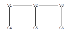
S1 has the lowest ID, and so becomes the root. S2 and S4 are directly connected, so they will enable the interfaces by which they reach S1 (Rule 1) while S1 will enable its interfaces by which S2 and S4 reach it (Rule 2).
S1 具有最低的 ID，因此成为根。S2 和 S4 是直接连接的，因此它们将启用它们到达 S1 的接口（规则 1），而 S1 将启用其 S2 和 S4 到达它的接口（规则 2）。

S3 has a unique lowest-cost route to S1, and so again by Rule 1 it will enable its interface to S2, while by Rule 2 S2 will enable its interface to S3.
S3 具有到 S1 的唯一最低成本路由，因此，根据规则 1，它将启用其到 S2 的接口，而根据规则 2，S2 将启用其到 S3 的接口。

S5 has two choices; it hears of equal-cost paths to the root from both S2 and S4. It picks the lower-numbered neighbor S2; the interface to S4 will never be enabled. Similarly, S4 will never enable its interface to S5.
S5 有两个选择;它听到从 S2 和 S4 到根的等价路径。它选择编号较低的邻居 S2;永远不会启用到 S4 的接口。同样，S4 永远不会启用其与 S5 的接口。

Similarly, S6 has two choices; it selects S3.
同样，S6 有两个选择;它选择 S3。

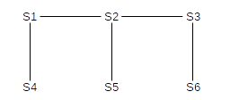
After these links are enabled (strictly speaking it is interfaces that are enabled, not links, but in all cases here either both interfaces of a link will be enabled or neither), the network in effect becomes:
启用这些链接后（严格来说，启用的是接口，而不是链接，但在所有情况下，链接的两个接口都将被启用，或者两者都不启用），网络实际上变为：

2.5.2 Example 2: Switches and Segments

2.5.2 示例 2：交换机和段

As an example involving switches that may join via unswitched Ethernet segments, consider the following network; S1, S2 and S3, for example, are all segment-neighbors via their common segment B. As before, the switch numbers represent their IDs. The letters in the clouds represent network segments; these clouds may include multiple hosts. Note that switches have no way to detect these hosts; only (as above) other switches.
例如，涉及可能通过非交换以太网分段加入的交换机，请考虑以下网络;例如，S1、S2 和 S3 都是通过其公共 Segment B 的 Segment 邻接方。和以前一样，交换机编号代表它们的 ID。云中的字母代表网络段;这些云可能包括多个主机。请注意，交换机无法检测这些主机;仅 （如上所述） 其他 Switch。

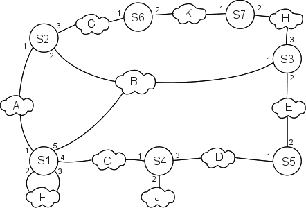
Eventually, all switches discover S1 is the root (because 1 is the smallest of {1,2,3,4,5,6}). S2, S3 and S4 are one (unique) hop away; S5, S6 and S7 are two hops away.
最终，所有开关都会发现 S1 是根（因为 1 是 {1,2,3,4,5,6} 的最小值）。S2、S3 和 S4 相距一个（唯一）跃点;S5、S6 和 S7 相距两个跃点。

Algorhyme （算法）

I think that I shall never see

a graph more lovely than a tree.

A tree whose crucial property

is loop-free connectivity.

A tree that must be sure to span

so packet can reach every LAN.

First, the root must be selected.

By ID, it is elected.

Least-cost paths from root are traced.

In the tree, these paths are placed.

A mesh is made by folks like me,

then bridges find a spanning tree.

Radia Perlman

算法（Algorhyme ）

我想我永远不会看到
比一棵树更可爱的图。
一棵树，它至关重要的特性
是无环连接性。
一棵树，它务必确保能够
让数据包到达每个局域网。
首先，必须选择根节点。
通过标识符，它被选中。
从根节点开始追踪最低成本路径。
在树中，这些路径被确定下来。
像我这样的人构建了一个网络，
然后网桥找出一棵生成树。
拉迪亚·珀尔曼

For the switches one hop from the root, Rule 1 enables S2’s port 1, S3’s port 1, and S4’s port 1. Rule 2 enables the corresponding ports on S1: ports 1, 5 and 4 respectively. Without the spanning-tree algorithm S2 could reach S1 via port 2 as well as port 1, but port 1 has a smaller number.
对于距离根一跃点的交换机，规则 1 启用 S2 的端口 1、S3 的端口 1 和 S4 的端口 1。规则 2 使能 S1 上的相应端口：分别是端口 1、5 和 4。如果没有生成树算法，S2 可以通过端口 2 和端口 1 到达 S1，但端口 1 的编号较小。

S5 has two equal-cost paths to the root: S5⟶S4⟶S1 and S5⟶S3⟶S1. S3 is the switch with the lower ID; its port 2 is enabled and S5 port 2 is enabled.
S5 有两条到根的等价路径：S5⟶S4⟶S1 和 S5⟶S3⟶S1。S3 是 ID 较低的交换机;其端口 2 已启用，S5 端口 2 已启用。

S6 and S7 reach the root through S2 and S3 respectively; we enable S6 port 1, S2 port 3, S7 port 2 and S3 port 3.
S6 和 S7 分别通过 S2 和 S3 到达根;我们启用了 S6 端口 1、S2 端口 3、S7 端口 2 和 S3 端口 3。

The ports still disabled at this point are S1 ports 2 and 3, S2 port 2, S4 ports 2 and 3, S5 port 1, S6 port 2 and S7 port 1.
此时仍处于禁用状态的端口是 S1 端口 2 和 3、S2 端口 2、S4 端口 2 和 3、S5 端口 1、S6 端口 2 和 S7 端口 1。

Now we get to Rule 3, dealing with how segments (and thus their hosts) connect to the root. Applying Rule 3,
现在我们来看看规则 3，处理 Segment（以及它们的主机）如何连接到根。应用规则 3，

• We do not enable S2 port 2, because the network (B) has a direct connection to the root, S1
  我们不启用 S2 端口 2，因为网络 （B） 与根 S1 有直接连接
• We do enable S4 port 3, because S4 and S5 connect that way and S4 is closer to the root. This enables connectivity of network D. We do not enable S5 port 1.
  我们确实启用了 S4 端口 3，因为 S4 和 S5 以这种方式连接，而 S4 更接近根。这将启用网络 D 的连接。我们不启用 S5 端口 1。
• S6 and S7 are tied for the path-length to the root. But S6 has smaller ID, so it enables port 2. S7’s port 1 is not enabled.
  S6 和 S7 在到根的路径长度上并列。但 S6 的 ID 较小，因此它启用了端口 2。S7 的端口 1 未启用。

Finally, Rule 4 enables S4 port 2, and thus connectivity for host J. It also enables S1 port 2; network F has two connections to S1 and port 2 is the lower-numbered connection.
最后，规则 4 启用 S4 端口 2，从而启用主机 J 的连接。它还启用 S1 端口 2;网络 F 有两个到 S1 的连接，端口 2 是编号较低的连接。

All this port-enabling is done using only the data collected during the root-discovery phase; there is no additional negotiation. The BPDU exchanges continue, however, so as to detect any changes in the topology.
所有这些端口启用都是仅使用在 root 发现阶段收集的数据完成的;没有额外的协商。但是，BPDU 交换将继续进行，以便检测拓扑中的任何更改。

If a link is disabled, it is not used even in cases where it would be more efficient to use it. That is, traffic from F to B is sent via B1, D, and B5; it never goes through B7. IP routing, on the other hand, uses the “shortest path”. To put it another way, all spanning-tree Ethernet traffic goes through the root node, or along a path to or from the root node.
如果禁用链接，则即使在使用效率更高的情况下也不会使用它。也就是说，从 F 到 B 的流量通过 B1、D 和 B5 发送;它永远不会通过 B7。另一方面，IP 路由使用 “最短路径”。换句话说，所有生成树以太网流量都通过根节点，或者沿着往返根节点的路径。

The traditional (IEEE 802.1D) spanning-tree protocol is relatively slow; the need to go through the tree-building phase means that after switches are first turned on no normal traffic can be forwarded for ~30 seconds. Faster, revised protocols have been proposed to reduce this problem.
传统的 （IEEE 802.1D） 生成树协议相对较慢;需要经历树构建阶段意味着在交换机首次打开后，在 ~30 秒内无法转发任何正常流量。已经提出了更快的修订协议来减少这个问题。

Another issue with the spanning-tree algorithm is that a rogue switch can announce an ID of 0, thus likely becoming the new root; this leaves that switch well-positioned to eavesdrop on a considerable fraction of the traffic. One of the goals of the Cisco “Root Guard” feature is to prevent this; another goal of this and related features is to put the spanning-tree topology under some degree of administrative control. One likely wants the root switch, for example, to be geographically at least somewhat centered.
生成树算法的另一个问题是，恶意交换机可以通告 ID 0，因此可能成为新的根;这使得该交换机处于有利位置，可以窃听相当大一部分流量。Cisco 的“Root Guard”功能的目标之一是防止这种情况;此功能和相关功能的另一个目标是将生成树拓扑置于某种程度的管理控制之下。例如，人们可能希望根开关至少在地理上处于中心位置。

2.6 Virtual LAN (VLAN)

2.6 虚拟局域网 （VLAN）

What do you do when you have different people in different places who are “logically” tied together? For example, for a while the Loyola University CS department was split, due to construction, between two buildings.
当你在不同的地方有不同的人“逻辑上”联系在一起时，你会怎么做？例如，由于施工原因，洛约拉大学计算机科学系曾一度被分成两座建筑。

One approach is to continue to keep LANs local, and use IP routing between different subnets. However, it is often convenient (printers are one reason) to configure workgroups onto a single “virtual” LAN, or VLAN. A VLAN looks like a single LAN, usually a single Ethernet LAN, in that all VLAN members will see broadcast packets sent by other members and the VLAN will ultimately be considered to be a single IP subnet (7.6 IP Subnets_). Different VLANs are ultimately connected together, but likely only by passing through a single, central IP router.
一种方法是继续将 LAN 保持在本地，并在不同子网之间使用 IP 路由。但是，将工作组配置到单个“虚拟”LAN 或 VLAN 上通常很方便（打印机是原因之一）。VLAN 看起来像单个 LAN，通常是单个以太网 LAN，因为所有 VLAN 成员都会看到其他成员发送的广播数据包，并且 VLAN 最终将被视为单个 IP 子网（7.6 个 IP 子网）。不同的 VLAN 最终会连接在一起，但可能只能通过单个中央 IP 路由器。

VLANs can be visualized and designed by using the concept of coloring. We logically assign all nodes on the same VLAN the same color, and switches forward packets accordingly. That is, if S1 connects to red machines R1 and R2 and blue machines B1 and B2, and R1 sends a broadcast packet, then it goes to R2 but not to B1 or B2. Switches must, of course, be told the color of each of their ports.
可以使用着色的概念来可视化和设计 VLAN。我们在逻辑上为同一 VLAN 上的所有节点分配相同的颜色，并相应地转发数据包。也就是说，如果 S1 连接到红色计算机 R1 和 R2 以及蓝色计算机 B1 和 B2，并且 R1 发送广播数据包，则它会发送到 R2，而不是 B1 或 B2。当然，必须告诉 Switch 每个端口的颜色。

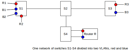
In the diagram above, S1 and S3 each have both red and blue ports. The switch network S1-S4 will deliver traffic only when the source and destination ports are the same color. Red packets can be forwarded to the blue VLAN only by passing through the router R, entering R’s red port and leaving its blue port. R may apply firewall rules to restrict red–blue traffic.
在上图中，S1 和 S3 分别具有红色和蓝色端口。交换机网络 S1-S4 仅在源端口和目标端口的颜色相同时传输流量。红色数据包只有通过路由器 R，进入 R 的红色端口，离开其蓝色端口，才能转发到蓝色 VLAN。R 可以应用防火墙规则来限制红蓝流量。

When the source and destination ports are on the same switch, nothing needs to be added to the packet; the switch can keep track of the color of each of its ports. However, switch-to-switch traffic must be additionally tagged to indicate the source. Consider, for example, switch S1 above sending packets to S3 which has nodes R3 (red) and B3 (blue). Traffic between S1 and S3 must be tagged with the color, so that S3 will know to what ports it may be delivered. The IEEE 802.1Q protocol is typically used for this packet-tagging; a 32-bit “color” tag is inserted into the Ethernet header after the source address and before the type field. The first 16 bits of this field is 0x8100, which becomes the new Ethernet type field and which identifies the frame as tagged.
当源端口和目标端口位于同一交换机上时，无需向数据包添加任何内容;交换机可以跟踪其每个端口的颜色。但是，必须额外标记 switch-to-switch 流量以指示源。例如，考虑上面的交换机 S1 将数据包发送到具有节点 R3（红色）和 B3（蓝色）的 S3。S1 和 S3 之间的流量必须标有颜色，以便 S3 知道它可能被传送到哪些端口。IEEE 802.1Q 协议通常用于此数据包标记;32 位“color”标记插入到 Ethernet 标头的源地址之后和 type 字段之前。此字段的前 16 位是 0x8100，它将成为新的 Ethernet type 字段，并将帧标识为已标记。

Double-tagging is possible; this would allow an ISP to have one level of tagging and its customers to have another level.
可以进行双重标记;这将允许 ISP 具有一个级别的标记，而其客户具有另一个级别。

2.7 Epilog

2.7 尾声

Ethernet dominates the LAN layer, but is not one single LAN protocol: it comes in a variety of speeds and flavors. Higher-speed Ethernet seems to be moving towards fragmenting into a range of physical-layer options for different types of cable, but all based on switches and point-to-point linking; different Ethernet types can be interconnected only with switches. Once Ethernet finally abandons physical links that are bi-directional (half-duplex links), it will be collision-free and thus will no longer need a minimum packet size.
以太网在 LAN 层占据主导地位，但不是一个单一的 LAN 协议：它有多种速度和风格。更高速以太网似乎正在朝着为不同类型电缆的一系列物理层选项发展，但所有这些都基于交换机和点对点链接;不同的以太网类型只能与交换机互连。一旦以太网最终放弃双向物理链路（半双工链路），它将无冲突，因此不再需要最小数据包大小。

Other wired networks have largely disappeared (or have been renamed “Ethernet”). Wireless networks, however, are here to stay, and for the time being at least have inherited the original Ethernet’s collision-management concerns.
其他有线网络已基本消失（或已更名为“以太网”）。然而，无线网络将继续存在，并且至少暂时继承了原始以太网的冲突管理问题。

2.8 Exercises

2.8 练习

1. Simulate the contention period of five Ethernet stations that all attempt to transmit at T=0 (presumably when some sixth station has finished transmitting). Assume that time is measured in slot times, and that exactly one slot time is needed to detect a collision (so that if two stations transmit at T=1 and collide, and one of them chooses a backoff time k=0, then that station will transmit again at T=2). Use coin flips or some other source of randomness.
2. 模拟五个以太网站的争用期，这些站都尝试以 T=0 进行传输（大概是当第六个站完成传输时）。假设时间以时隙时间来测量，并且正好需要一个时隙时间来检测冲突（因此，如果两个站在 T=1 处传输并发生碰撞，并且其中一个站选择退避时间 k=0，则该站将在 T=2 处再次传输）。使用硬币翻转或其他一些随机性来源。
3. Suppose we have Ethernet switches S1 through S3 arranged as below. All forwarding tables are initially empty.
4. 假设我们有以太网交换机 S1 到 S3，排列如下。所有转发表最初都是空的。

S1────────S2────────S3───D
│     │     │
A     B     C

(a). If A sends to B, which switches see this packet?

(b). If B then replies to A, which switches see this packet?

©. If C then sends to B, which switches see this packet?

(d). If C then sends to D, which switches see this packet?

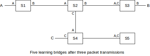
3. Suppose we have the Ethernet switches S1 through S4 arranged as below. All forwarding tables are empty; each switch uses the learning algorithm of 2.4 Ethernet Switches_.
4. 假设我们有以太网交换机 S1 到 S4，排列如下。所有转发表都为空;每个交换机都使用 2.4 以太网交换机的学习算法。

       B
       │
       S4
       │
A───S1────────S2────────S3───C
       │
       D

Now suppose the following packet transmissions take place:
现在假设发生了以下数据包传输：

• A sends to B A 向 B 发送
• B sends to A B 发送到 A
• C sends to B C 向 B 发送
• D sends to A D 发送到 A

For each switch, list what source nodes (eg A,B,C,D) it has seen (and thus learned about).
对于每个 switch，列出它看到（并因此了解）的源节点（例如 A、B、C、D）。

4. In the switched-Ethernet network below, find two packet transmissions so that, when a third transmission A⟶D occurs, the packet is delivered to B (that is, it is forwarded out all ports of S2), but is not similarly delivered to C. All forwarding tables are initially empty, and each switch uses the learning algorithm of 2.4 Ethernet Switches_.
5. 在下面的交换以太网网络中，找到两个数据包传输，这样，当发生第三次传输 A⟶D 时，数据包被传送到 B（即，它被转发出 S2 的所有端口），但不会以类似的方式传送到 C。所有转发表最初都是空的，每个交换机都使用 2.4 以太网交换机的学习算法。

       B     C
       │     │
A───S1────────S2────────S3───D

Hint: Destination D must be in S3’s forwarding table, but must not be in S2’s.
提示：目标 D 必须位于 S3 的转发表中，但不能位于 S2 的转发表中。

5. Given the Ethernet network with learning switches below, with (disjoint) unspecified parts represented by ?, explain why it is impossible for a packet sent from A to B to be forwarded by S1 only to S2, but to be forwarded by S2 out all of S2’s other ports.
6. 给定下面带有学习开关的以太网网络，其中（不相交的）未指定部分用 ？表示，解释为什么从 A 发送到 B 的数据包不可能只由 S1 转发到 S2，而不能由 S2 从 S2 的所有其他端口转发出去。

  ?     ?
  |     |
A───S1────────S2───B

6. In the diagram of 2.4 Ethernet Switches*_, suppose node D is connected to S5, and, with the tables as shown below the diagram, D sends to B.
7. 在 2.4 以太网交换机的示意图中，假设节点 D 连接到 S5，并且根据下图所示的表格，D 发送到 B。

(a). Which switches will see this packet, and thus learn about D?

(b). Which of the switches in part (a) do not already know where B is (and will thus forward the packet out all non-arrival interfaces)?

7. Suppose two Ethernet switches are connected in a loop as follows; S1 and S2 have their interfaces 1 and 2 labeled. These switches do not use the spanning-tree algorithm.
8. 假设两台以太网交换机连接成一个回路，如下所示;S1 和 S2 的接口 1 和 2 已标记。这些交换机不使用生成树算法。

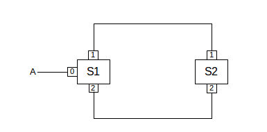
Suppose A attempts to send a packet to destination B, which is unknown. S1 will therefore forward the packet out interfaces 1 and 2. What happens then? How long will A’s packet circulate?
假设 A 尝试将数据包发送到未知的目标 B。因此，S1 将转发数据包传出接口 1 和 2。然后会发生什么？A 的数据包会流通多长时间？

8. The following network is like that of 2.5.1 Example 1: Switches Only_, except that the switches are numbered differently. What is the end result of the spanning-tree algorithm in this case?
9. 以下网络类似于 2.5.1 示例 1：仅交换机，只是交换机的编号不同。在这种情况下，生成树算法的最终结果是什么？

S1──────S4──────S6
│    │    │
│    │    │
│    │    │
S3──────S5──────S2

9. Suppose you want to develop a new protocol so that Ethernet switches participating in a VLAN all keep track of the VLAN “color” associated with every destination. Assume that each switch knows which of its ports (interfaces) connect to other switches and which may connect to hosts, and in the latter case knows the color assigned to that port.
10. 假设您要开发一种新协议，以便参与 VLAN 的以太网交换机都跟踪与每个目的地关联的 VLAN“颜色”。假设每个交换机都知道其哪些端口（接口）连接到其他交换机，哪些端口（接口）可以连接到主机，在后一种情况下，知道分配给该端口的颜色。

---

1. The Core Reason: Collision Detection in CSMA/CD

The primary reason for the minimum Ethernet frame size of 64 bytes is related to collision detection in networks using CSMA/CD (Carrier Sense Multiple Access with Collision Detection).
以太网最小帧大小为 64 字节的主要原因是与使用 CSMA/CD（具有冲突检测的载波侦听多路访问）的网络中的冲突检测有关。

CSMA/CD requires a sending station to be able to detect a collision during the entire transmission of the frame.
CSMA/CD 要求发送站能够在整个帧的传输过程中检测到冲突。

2. Collision Window and Propagation Delay

The minimum frame size is designed to be long enough to ensure that the sender transmits for at least twice the maximum one-way propagation delay (round-trip time) of the network.
最小帧大小的设计要足够长，以确保发送方传输的时间至少是网络最大单向传播延迟（往返时间）的两倍。

This “collision window” gives the sender enough time to detect a collision signal from the farthest point on the network before it finishes transmitting the frame.
这个“冲突窗口”为发送方提供了足够的时间，在完成帧传输之前检测到来自网络最远点的冲突信号。

3. How it Works

If a sending station finishes transmitting a frame *before* the maximum round-trip time has elapsed, it wouldn’t be able to detect a collision that occurred far away on the network.
如果发送站在最长往返时间过去之前完成帧传输，它将无法检测到发生在网络远处的冲突。

By enforcing a minimum frame size, the network ensures that the sender will still be listening for collisions when the collision signal arrives.
通过强制执行最小帧大小，网络确保发送方在冲突信号到达时仍会监听冲突。

4. Calculating the Minimum Size

The 64-byte minimum frame size is derived from the maximum allowed network diameter and the signal propagation speed through the cable.
64 字节的最小帧大小来自最大允许网络直径和信号通过电缆的传播速度。

It’s a compromise based on the limitations of early Ethernet technology.
这是基于早期以太网技术的限制所做的折衷。

5. Full-Duplex and Modern Networks

In modern, switched, full-duplex Ethernet networks, CSMA/CD is not used, and collisions are greatly reduced.
在现代、交换、全双工以太网网络中，不使用 CSMA/CD，并且大大减少了冲突。

However, the minimum frame size is still enforced for compatibility reasons and to avoid issues with devices that might still rely on the minimum size assumption.
但是，出于兼容性原因以及避免可能仍然依赖于最小尺寸假设的设备出现问题，仍然强制执行最小帧大小。

6. Padding

If the data to be sent is less than the minimum frame size, the Ethernet controller adds padding to bring the frame up to the required size.
如果要发送的数据小于最小帧大小，以太网控制器会添加填充以使帧达到所需的大小。

This padding is transparent to the application layer.
这种填充对应用层是透明的。

---

1. The 64-Byte Minimum Ethernet Frame Size Rule:

The Ethernet standard specifies a minimum frame size of 64 bytes (including the header, data, and FCS).
以太网标准规定了最小帧大小为 64 字节（包括头部、数据和 FCS）。

This minimum size is related to collision detection in legacy Ethernet networks (CSMA/CD).
这个最小尺寸与传统以太网网络 (CSMA/CD) 中的冲突检测有关。

It ensures that a sending station transmits for a sufficient amount of time to detect collisions that might occur on the network.
它确保发送站传输足够长的时间，以便检测可能发生在网络上的冲突。

2. Padding and Short Frames:

If the data portion of a frame is less than the required minimum, the sending network interface card (NIC) will add padding to bring the frame up to 64 bytes.
如果帧的数据部分小于要求的最小值，则发送网络接口卡 (NIC) 将添加填充，使帧达到 64 字节。

This padding is usually added at the MAC layer.
此填充通常在 MAC 层添加。

Therefore, you typically won’t see frames smaller than 64 bytes on the wire in a correctly functioning network.
因此，在正常运行的网络中，您通常不会在网络上传输小于 64 字节的帧。

3. Exceptions and Violations:

Malformed or corrupted frames can violate this rule.
格式错误或损坏的帧可能会违反此规则。

Early switches sometimes had issues and could forward undersized frames (runt frames).
早期的交换机有时会出现问题，可能会转发过小的帧（残帧）。

Network analysis tools might capture frames smaller than 64 bytes if they are capturing at a point where the frame is corrupted or incomplete.
网络分析工具可能会捕获小于 64 字节的帧，如果在帧损坏或不完整时捕获。

Sometimes, protocols might encapsulate smaller packets within Ethernet, but the *Ethernet frame* itself should still be at least 64 bytes due to padding.
有时，协议可能会将较小的包封装在以太网中，但由于填充，以太网帧本身仍然至少为 64 字节。

4. Modern Networks and Full-Duplex:

In modern, switched, full-duplex Ethernet networks, collisions are much less of a concern.
在现代的、交换的、全双工以太网网络中，冲突不再是一个大问题。

However, the 64-byte minimum frame size rule is still generally enforced to maintain compatibility and proper operation.
然而，为了保持兼容性和正常运行，通常仍然强制执行 64 字节的最小帧大小规则。

5. Importance of FCS (Frame Check Sequence):

The FCS (Frame Check Sequence) is a checksum appended to the Ethernet frame to detect errors in transmission.
FCS（帧校验序列）是一个附加到以太网帧的校验和，用于检测传输中的错误。

It’s a crucial part of the Ethernet frame structure, ensuring data integrity.
它是以太网帧结构的重要组成部分，可确保数据完整性。

6. Runt Frames:

“Runt frames” are Ethernet frames that are smaller than the minimum size of 64 bytes. These are considered invalid.
“残帧”是指小于 64 字节最小尺寸的以太网帧。这些被认为是无效的。

Runt frames are usually discarded by network devices.
残帧通常会被网络设备丢弃。

---

1. Fragment-Free Switching Overview

Fragment-Free switching aims to reduce bad frame forwarding.
无碎片交换旨在减少错误帧的转发。

It checks the first 64 bytes of the frame before forwarding.
它在转发帧之前检查帧的前 64 个字节。

This ensures that the frame has passed the collision window.
这确保了帧已经通过了冲突窗口。

2. Addressing Collision Issues

Collisions are most likely to occur in the first 64 bytes of a frame.
冲突最有可能发生在帧的前 64 个字节中。

By checking these 64 bytes, Fragment-Free switching avoids forwarding frames damaged by early collisions.
通过检查这 64 个字节，无碎片交换避免了转发被早期冲突损坏的帧。

3. Trade-off: Latency vs. Error Reduction

Fragment-Free switching offers a compromise between store-and-forward (higher latency, better error checking) and cut-through switching (lower latency, less error checking).
无碎片交换提供了存储转发（延迟较高，错误检查更好）和直通交换（延迟较低，错误检查较少）之间的折衷方案。

It has lower latency than store-and-forward because it doesn’t wait for the entire frame.
它的延迟低于存储转发，因为它不需要等待整个帧。

It has better error reduction than cut-through because it checks the first 64 bytes.
它的错误减少优于直通交换，因为它检查了前 64 个字节。

4. Why 64 Bytes?

The 64-byte check corresponds to the minimum Ethernet frame size required to detect collisions on a network using CSMA/CD.
64 字节的检查对应于使用 CSMA/CD 的网络上检测冲突所需的最小以太网帧大小。

If a collision occurs, it should be detected within the first 64 bytes.
如果发生冲突，应该在前 64 个字节内检测到。

This is related to the round-trip time (RTT) of the network.
这与网络的往返时间 (RTT) 有关。

5. Considered Obsolete

Fragment-Free switching is largely obsolete in modern networking environments.
无碎片交换在现代网络环境中已基本过时。

Full-duplex Ethernet and switched networks have made collisions much less frequent.
全双工以太网和交换网络使得冲突发生的频率大大降低。

Modern switches typically use store-and-forward or cut-through switching, and the performance difference due to fragment-free switching is negligible.
现代交换机通常使用存储转发或直通交换，并且由于无碎片交换引起的性能差异可以忽略不计。

6. Related Concepts

Store-and-Forward Switching: Stores the entire frame before forwarding.
存储转发交换：在转发之前存储整个帧。

Cut-Through Switching: Forwards the frame as soon as the destination address is read.
直通交换：读取到目标地址后立即转发帧。

Collision Domain: A network segment where devices compete for access to the medium, and collisions can occur.
冲突域：设备竞争访问介质并且可能发生冲突的网络段。

CSMA/CD (Carrier Sense Multiple Access with Collision Detection): A media access control method used in early Ethernet to detect and handle collisions.
具有冲突检测的载波侦听多路访问 (CSMA/CD)：早期以太网中使用的一种媒体访问控制方法，用于检测和处理冲突。

---

以太网最小帧长为什么是 64 字节

引言

在以太网环境中，RFC2544 规定了测试时数据包的长度应为 64、128、256、512、1024、1280、1518 字节（“Frame sizes to be used on Ethernet:64, 128, 256, 512, 1024, 1280, 1518”）。本文对以太网最小帧长的来源进行详细讨论。

一、以太网（IEEE 802.3）帧格式

1. 前导码：7 字节 0x55，一串 1、0 间隔，用于信号同步
2. 帧起始定界符：1 字节 0xD5（10101011），表示一帧开始
3. 目的 MAC 地址：6 字节
4. 源 MAC 地址：6 字节
5. 类型/长度：2 字节，0～1500 表示长度域值，1536～65535（0x0600～0xFFFF）表示类型域值
6. 数据：46～1500 字节
7. 帧校验序列（FCS）：4 字节，使用 CRC 算法计算从目的 MAC 到数据域的校验和

二、最小帧长的理论基础

以太网采用 CSMA/CD 作为介质访问控制算法，包括"先听后发、边听边发、随机延迟后重发"等冲突避免机制。为确保冲突检测有效，必须规定最小帧长。

极限情况分析

考虑以下场景：当主机 A 发送的帧还未传输到主机 B 的前一刻，B 开始发送帧。当 A 的帧到达 B 时，B 检测到冲突并发送冲突信号。如果 A 在接收到冲突信号之前已完成发送，则 A 将无法检测到冲突，误认为发送成功。

根据标准，10Mbps 以太网采用中继器时，最大连接长度为 2500 米，最多经过 4 个中继器。因此，规定 10Mbps 以太网一帧的最小发送时间为 51.2 微秒，即 512 位时间（512 位 = 64 字节）。这个时间定义为"以太网时隙"或"冲突时槽"。

• 100Mbps 以太网的时隙仍为 512 位时（5.12μs）
• 1000Mbps 以太网的时隙增至 512 字节（4096 位时，4.096μs）

三、碰撞槽时间的数学模型

假设：

• $S$：公共总线媒体长度
• $0.7C$：帧在媒体上的传播速度（光速的 0.7 倍）
• $R$：网络的传输率（bps）
• $L$：帧长（bits）
• $t_{PHY}$：物理层时延

则有：

碰撞槽时间 $=\frac{2S}{0.7C}+2t_{PHY}$

因为 $\frac{L_{min}}{R}=$ 碰撞槽时间

所以：$L_{min}=\left(\frac{2S}{0.7C}+2t_{PHY}\right)\times R$

其中 $L_{min}$ 为最小帧长度。

碰撞槽时间的特性

1. 它是检测一次碰撞所需的最长时间
2. 它决定了帧长度的下限（最短帧长）
3. 发生碰撞时会产生帧碎片
4. 如发生碰撞，需等待时间 $t=rT$（$T$ 为碰撞槽时间）

最坏情况的冲突检测

1. 假设网络中相距最远的两个主机 A 和 B 之间的信号传播时延为 $\tau$
2. 主机 A 在 $t$ 时刻开始发送，数据帧在 $t+\tau$ 时刻到达 B
3. 若 B 在 $t+\tau -\epsilon$ 时刻开始发送，则 B 在 $t+\tau$ 时检测到冲突并发出阻塞信号
4. 阻塞信号将在 $t+2\tau$ 时到达 A，因此 A 必须在 $t+2\tau$ 时仍在发送才能检测到冲突
5. 帧的发送时间必须大于 $2\tau$

根据标准，10Mbps 以太网中，最小发送时间为 51.2μs，即 512 位时间，因此最小帧长为 64 字节。

四、扩展模型

更完整的模型可表示为：

$\frac{L_{min}}{R}=\frac{2\times S}{0.7\times C}+2\times T_{phy}+n\times T_r$

其中：

• $L_{min}$：最小帧长
• $R$：网络速率（如 10Mbps）
• $S$：碰撞域直径（$\times 2$ 表示信号往返时间）
• $C$：光速（$\times 0.7$ 表示在双绞线中的传播速度）
• $T_{phy}$：物理层延时（$\times 2$ 表示经过发送和接收两个物理层）
• $T_r$：中继器延时（通常相当于两个物理层的延时）
• $n$：中继器数量

实例计算

根据 IEEE 802.3 标准，$L_{min}=64$ 字节；

设 $R=10\text{ Mbps}$，$T_{phy}=15\text{ μs}$，$T_r=0$，

则可计算出 $S\approx 2.3\text{ km}$

五、最大传输单元（MTU）

以太网规定最大传输单元为 1518 字节，其中包含 14 字节的以太网帧头（目的 MAC 地址 + 源 MAC 地址 + 类型/长度字段）和 4 字节的帧校验序列，因此数据部分的最大长度为 1500 字节。

制定最大传输单元的考虑因素：

1. 避免过长帧导致的高重传成本
2. 减轻网络设备的处理负担
3. 适应不同链路层技术的兼容性需求
4. 在常见网络应用场景下保证传输效率

六、以太网标准的演进

IEEE 802.3 标准于 1983 年 6 月 24 日首次发布，随后获得 ANSI 和 ISO 认可。尽管早期与 Ethernet II 标准并存，但在 1998 年编辑的 IEEE 802.3-2002 版本中进行了重大改进，使其具备了 Ethernet II 的灵活性，最终成为以太网的唯一标准。

IEEE 802.3-2002 标准定义了以太网的头结构为：目的地址(6) + 源地址(6) + 长度/类型(2) = 14 字节。

2005 年以后，IEEE 继续制定 802.3 标准的新版本，不断适应网络技术的发展需求。

结论：

以太网最小帧长 64 字节是由以太网帧的基本结构组成：目的 MAC 地址（6 字节）+ 源 MAC 地址（6 字节）+ 类型字段（2 字节）+ CRC 校验（4 字节）= 18 字节，再加上最小数据载荷 46 字节，总计 64 字节。

参考文献

1. RFC2544: Benchmarking Methodology for Network Interconnect Devices.

2. IEEE 802.3: Ethernet Standards.

---

Fragment Free 模式为何只取前 64 字节

发布时间：(2006-10-03 07:40:03)

已知交换机存在三种转发模式：Cut-Through、Fragment Free、Store and Forward。每种模式均具有特定意义。在此探讨 Fragment Free 模式取值为 64 字节的原因，首先查看相关图示（见图 1）。

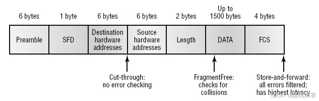
一、Cut-Through 模式

该模式仅读入目的 MAC 地址，其延迟最小，但无法进行错误检测。部分交换机支持在每端口基础上设置错误门限值（error threshold），当错误数量超过此自定义值时，端口将自动从 Cut-Through 模式切换至 Store and Forward 模式。若端口在一定时间内运行正常，可再次切换回 Cut-Through 模式。而 Store and Forward 模式具备错误检测功能，能够快速发现问题。

二、Fragment Free 模式

Fragment Free 又称 Modified Cut-Through。交换机在该模式下会读至冲突窗口（64 字节）。这是因为若数据包因冲突产生错误，大多发生在 64 字节以内。在此模式下，会持续检测至数据部分，以确定不存在分片（fragmentation）。Fragment Free 模式在提供较好错误检测能力的同时，几乎未增加延迟。思科 1900 系列交换机默认采用此模式。

三、Store and Forward 模式

此模式为思科主流交换机的首选方案。交换机将整个帧拷贝至板载缓存中，并进行 CRC 校验。由于需处理整个帧，其延迟长短与帧大小成正比。若帧包含 CRC 错误、长度过短（小于 64 字节）或过长（大于 1518 字节），均会被丢弃。

---

References

• 2 Ethernet — An Introduction to Computer Networks
  https://intronetworks.cs.luc.edu/1/html/ethernet.html

• What exactly is fragment free switching?

• Is the 64-byte minimal Ethernet packet rule respected in practice?

• Why does ethernet have a minimum frame size specified?

• 以太网最小帧长为什么是64字节 - hotty - 博客园
  https://www.cnblogs.com/happyhotty/articles/2220203.html

• Fragment Free 模式为何只取前 64 字节_Jackson_新浪博客
  https://blog.sina.com.cn/s/blog_56fdccdb010006al.html