计算机视觉--基本的图像操作和处理

最新推荐文章于 2022-07-05 23:05:39 发布

原创最新推荐文章于 2022-07-05 23:05:39 发布 · 524 阅读

0 ·

CC 4.0 BY-SA版权

本文详细介绍图像处理中的关键概念和技术，包括图像直方图的绘制、直方图均衡化的实现及效果展示，以及高斯模糊的应用。通过Python代码实例，深入浅出地讲解了图像处理的基本操作，适合初学者入门。

第一章基本的图像操作和处理

（一）图像直方图

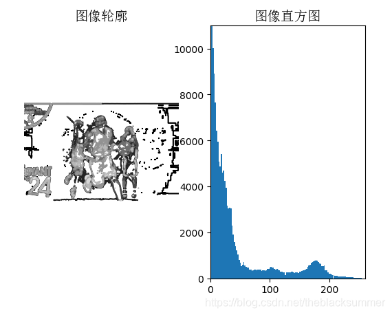
图像的直方图用来表征该图像像素值得分布情况。

代码：

from PIL import Image
from pylab import *

from matplotlib.font_manager import FontProperties
font = FontProperties(fname=r"c:\windows\fonts\SimSun.ttc", size=14)
im = array(Image.open(‘X.jpg’).convert(‘L’)) # 打开图像，并转成灰度图像

figure()
subplot(121)
gray()
contour(im, origin=‘image’)
axis(‘equal’)
axis(‘off’)
title(u’图像轮廓’, fontproperties=font)

subplot(122)
hist(im.flatten(), 128)
title(u’图像直方图’, fontproperties=font)
plt.xlim([0,260])
plt.ylim([0,11000])

show()

python和matlab之间的区别。在matlab中使用imshow就可以直接将图片显示出来，而在python中，需要写一个函数show来显示图片

运行结果如下：

在这里插入图片描述

（二）直方图均衡化

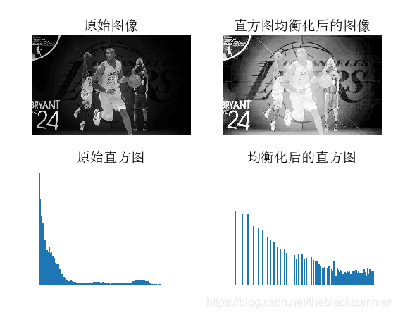
直方图均衡化是指将一幅图像的灰度直方图变平，使变换后的图像中每个灰度值的分布概率都相同。

代码：

from PIL import Image
from pylab import *
from PCV.tools import imtools

from matplotlib.font_manager import FontProperties
font = FontProperties(fname=r"c:\windows\fonts\SimSun.ttc", size=14)

im = array(Image.open(‘X.jpg’).convert(‘L’)) # 打开图像，并转成灰度图像
#im = array(Image.open(‘X.jpg’).convert(‘L’))
im2, cdf = imtools.histeq(im)

figure()
subplot(2, 2, 1)
axis(‘off’)
gray()
title(u’原始图像’, fontproperties=font)
imshow(im)

subplot(2, 2, 2)
axis(‘off’)
title(u’直方图均衡化后的图像’, fontproperties=font)
imshow(im2)

subplot(2, 2, 3)
axis(‘off’)
title(u’原始直方图’, fontproperties=font)
#hist(im.flatten(), 128, cumulative=True, normed=True)
hist(im.flatten(), 128, normed=True)

subplot(2, 2, 4)
axis(‘off’)
title(u’均衡化后的直方图’, fontproperties=font)
#hist(im2.flatten(), 128, cumulative=True, normed=True)
hist(im2.flatten(), 128, normed=True)

show()

运行结果如下：
在这里插入图片描述

（三）高斯模糊

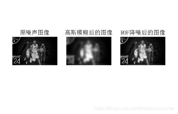
图像的高斯模糊是一个非常经典的图像卷积例子。

代码：

from PIL import Image
from pylab import *
from numpy import *
from numpy import random
from scipy.ndimage import filters
from scipy.misc import imsave
from PCV.tools import rof

“”" This is the de-noising example using ROF in Section 1.5. “”"

font = FontProperties(fname=r"c:\windows\fonts\SimSun.ttc", size=14)

im = array(Image.open(‘X.jpg’).convert(‘L’))

U,T = rof.denoise(im,im)
G = filters.gaussian_filter(im,10)

#imsave(‘synth_original.pdf’,im)
#imsave(‘synth_rof.pdf’,U)
#imsave(‘synth_gaussian.pdf’,G)

figure()
gray()

subplot(1,3,1)
imshow(im)
#axis(‘equal’)
axis(‘off’)
title(u’原噪声图像’, fontproperties=font)

subplot(1,3,2)
imshow(G)
#axis(‘equal’)
axis(‘off’)
title(u’高斯模糊后的图像’, fontproperties=font)

subplot(1,3,3)
imshow(U)
#axis(‘equal’)
axis(‘off’)
title(u’ROF降噪后的图像’, fontproperties=font)

show()

运行结果如下：
在这里插入图片描述