


A Fast Diagnosis Scheme for Multiple Switch Faults in Cascaded H-Bridge Multilevel Converters
Dong Xie, Graduate Student Member, IEEE, Chunxu Lin, Student Member, IEEE, Qingli Deng, Student Member, IEEE, Xinglai Ge, Member, IEEE, and Bin Gou, Member, IEEE
Abstract —The increasing importance of cascaded H-bridge multilevel converters(CHBMCs) in high-power applications requires a higher priority to detect and protect against fault conditions. In this paper, a current residual-based diagnosis scheme is proposed for the CHBMCs without additional sensors. On the premise of filtering the sampled DC voltages, comparing the calculated actual values of output current with the expected values in the control system, normalized diagnostic variables are established to localize single or multiple open-circuit switches. Benefit from the diagnostic variables corresponding directly to the switches of each H-bridge, this method can be easily extended to the CHBMCs with arbitrary submodules. Furthermore, the parameter estimation and enhanced detection algorithm are introduced to ensure the immunity of the diagnostic method to the large parameter changes and measurement noises. The faulty component can be accurately diagnosed within one line cycle regardless of the faulty modules and operating conditions. The effectiveness of the proposed method is substantiated using experimental results from the hardware platform of the CHBMCs.
Index Terms —Fault diagnosis, open-circuit fault, cascaded H-bridge multilevel converters (CHBMCs), current residual.
I. INTRODUCTION
Cascaded H-bridge multilevel converters (CHBMCs) have become an important topology in high-power applications such as grid-connected converters, voltage source inverters, and solid-state transformers (SST) due to their advantages of fast dynamic response, high efficiency, and flexible scalability [1]–[3]. This paper focuses on single-phase cascaded H-bridge multilevel converters (single-phase CHBMCs), which have broad application prospects in train sets equipped with medium-frequency transformers (MFTs) [4]. Taking the traction drive system with medium-frequency transformers (MFTs) as an example, as shown in Fig. 1, the cascaded H-bridge multilevel converter (CHBMCs) is used as the input stage to regulate power flow and maintain the DC-link voltage. Each H-bridge is connected via a medium-frequency transformer (MFT) to a dual-active bridge converter (DAB converter), achieving power transmission and electrical isolation between the cascaded H-bridge stage and the traction load.
Various control techniques have been studied, mainly focusing on voltage balance control of multiple H-bridge units and power distribution performance of output parallel DAB converters [5]–[7]. With the increasing importance of cascaded H-bridge multilevel converters in high-power applications, higher safety and priority requirements for detecting and protecting against fault conditions are receiving growing attention. The large number of switches in cascaded H-bridge multilevel converters operating for long periods under high power and complex environments leads to a high probability of switch failures. To address this issue, fault-tolerant control schemes have been proposed to maintain safe operation of the system under internal fault conditions [8]–[10]. Prior to that, early fault detection and localization are crucial to avoid secondary failures of other components and reduce economic losses to the system.
For switches in cascaded H-bridge multilevel converters, catastrophic failure behaviors can be roughly divided into short-circuit faults and open-circuit faults. Short-circuit faults caused by thermal runaway or thermal shock are destructive and typically use hardware protection to ensure a short-circuit detection time (within 10 microseconds) [11]. However, open-circuit faults caused by bond wire detachment or gate driver failure [12],[13], may not immediately cause system shutdown and might remain undetected for a long time. Long-term operation could subject other cells to higher thermal stress and trigger chain failures. Therefore, accurate and fast diagnostic algorithms for open-circuit faults have been widely studied in multilevel converters.
In recent years, fault detection and localization methods for modular multilevel converters (MMC) have been widely proposed [14]–[19]. Considering that the submodules (SM) in each arm of the MMC are connected in series, the capacitor voltage of a faulty submodule will exhibit corresponding fault characteristics. Thus, these characteristics are often selected as fault detection variables to locate faulty switches. Some detection methods, such as measuring arm voltages and adding extra hardware circuits [14],[15], have not been widely applied due to high system cost and measurement difficulty. In contrast, model-based methods, such as sliding mode observers [16] and Kalman filter-based observers [17], are used to locate faulty submodules or faulty switches. These methods estimate certain state variables (e.g., grid current, capacitor voltage) based on drive signals and system models. However, their detection time exceeds 50ms. Additionally, some literature explores model predictive control (MPC)-based methods [18],[19], by estimating the actual sum and difference of upper and lower arm voltages and comparing them with the corresponding values output by the controller, allowing fault switch localization within a fundamental cycle. However, this method does not consider simultaneous multiple fault scenarios.
Unlike modular multilevel converters using half-bridge submodules, cascaded H-bridge multilevel converters have more switches, and different switches in one or more H-bridges may exhibit similar fault characteristics, posing a major challenge for fault diagnosis. In [20], current waveforms and zero-voltage switching states are analyzed, but require more than two fundamental cycles to locate the fault. Considering that the input-side voltage contains voltage state information from different H-bridges, literature [21]–[24] proposes a series of voltage analysis-based diagnostic algorithms. High-frequency harmonic analysis and principal component analysis (PCA) are used to directly extract voltage fault features [21],[22], but require additional voltage sensors. By measuring the terminal voltage of the H-bridge and comparing the estimated voltage with the measured value, fault detection is achieved [23],[24]. Although the method proposed in [23] requires only 2n measurement cycles (n being the number of H-bridges) for single-switch faults, multiple fault detection may require higher computational time. Literature [24] achieves an improved method but requires obtaining switching moments where only one H-bridge performs switching operations, and the modulation method changes during fault localization, which may increase diagnostic complexity and localization time in cases with more H-bridges. Specific individual or multiple fault switches cannot be identified.
Additionally, diagnosis methods based on mixed logical dynamic (MLD) models have been successfully applied to fault diagnosis of single-phase PWM converters [25]–[27]. For single-phase cascaded H-bridge multilevel converters, an integral sliding mode observer containing numerous tuning parameters is designed [28] to analyze the DC component of the fault profile, where the selection of observer gain is relatively complex. By analyzing the residual characteristics of grid current and DC-link voltage, the method proposed in [29] has faster detection speed and can directly locate the faulty switch. However, it can only detect a single faulty switch, and diagnostic accuracy may be affected by noise interference and parameter variations. The output current of each H-bridge contains individual characteristic information of each H-bridge, making it possible to detect and locate multiple faults in single or multiple H-bridges [30]. By comparing predicted grid current with measured current in a model predictive controller, multiple faults are detected, and a fault location matrix is designed to locate faults in [31]. However, the update of fault location variables is relatively complex, and the impact of large parameter changes and measurement noise on the diagnostic algorithm is not considered, which are important issues affecting diagnostic robustness in high-power systems.
Inspired by the above discussions, this paper proposes an improved and extended version of the technique described in [30]. First, by analyzing the H-bridge structure and related signals in the control system, the actual output current and expected output current of each H-bridge are obtained. Normalized diagnostic variables for different switches are established to simplify threshold setting and improve the universality of the diagnostic algorithm. Additionally, a filtering method based on nonlinear functions is adopted to reduce the impact of measurement noise. Parameter estimation and enhanced detection algorithms are introduced to further improve the anti-interference capability of the diagnostic method. Finally, an experimental platform for the cascaded H-bridge multilevel converter is built to verify the effectiveness and robustness of the proposed method.
II. DESCRIPTION AND MODELING OF CASCADED H-BRIDGE MULTILEVEL CONVERTERS
A. Overview of Cascaded H-Bridge Multilevel Converters
Figure 2 shows the main circuit of a single-phase cascaded H-bridge multilevel converter, consisting of n H-bridges connected in series. Each H-bridge has a DC-link capacitor Ci, an equivalent load Ri, and four switches, namely Ti1, Ti2, Ti3, and Ti4. uN and iN are the grid voltage and grid current, respectively. LN and RN are the filter inductor and parasitic resistance, respectively. iouti, ici, and ioi are the output current, current through capacitor Ci, and load current of each H-bridge, respectively.
A typical voltage-current double-loop controller is usually employed to maintain the DC-link voltage ui near its reference value and achieve a power factor close to unity at the input side of the cascaded H-bridge multilevel converter. Simultaneously, a DC-capacitor voltage balancing scheme is implemented to ensure equal DC-link voltages across all units, thus quickly correcting deviations among different DC-link voltages.
B. Mixed Logical Dynamic Model and Residual Generation of Cascaded H-Bridge Multilevel Converters
The cascaded H-bridge multilevel converter, possessing continuous current/voltage signals and discrete switching signals, is regarded as a typical hybrid system. Define two arm switching functions Sia and Sib; the switching state of any switch or freewheeling diode can be described as:
$$
\begin{cases}
S_{ia} = 1, \text{ if } T_{i1} \text{ or } D_{i1} \text{ is on}, \
S_{ia} = 0, \text{ if } T_{i2} \text{ or } D_{i2} \text{ is on},
\end{cases}
\quad
\begin{cases}
S_{ib} = 1, \text{ if } T_{i3} \text{ or } D_{i3} \text{ is on}, \
S_{ib} = 0, \text{ if } T_{i4} \text{ or } D_{i4} \text{ is on},
\end{cases}
\quad (i=1,2,…,n)
\tag{1}
$$
Given the drive signals of the switches (si1-si4), λ is used to describe the direction of the grid current, where λ=1 indicates iN>0, otherwise λ=0. According to the modeling analysis in [29], expressions for Sia and Sib can be obtained:
$$
\begin{cases}
S_{ia} = s_{i1}\lambda + s_{i2}\bar{\lambda} \
S_{ib} = s_{i3}\lambda + s_{i4}\bar{\lambda}
\end{cases}
\tag{2}
$$
where $\bar{\lambda}$ is the logical inversion of λ, $s_{i2}$ and $s_{i4}$ are the logical inversions of the corresponding variables.
Mixed Logical Dynamic (MLD) modeling considers switch dead-time and switching states while ignoring other characteristics such as conduction resistance and forward voltage drop [26]. According to Kirchhoff’s circuit laws, the differential equations for grid current and DC-link voltage can be expressed as:
$$
\begin{cases}
L_N \frac{di_N}{dt} = u_N - R_N i_N - \sum_{i=1}^{n}(S_{ia} - S_{ib})u_i \
C_i \frac{du_i}{dt} = i_{ci} - i_{oi}
\end{cases}
\tag{3}
$$
Based on the discrete nature of the controller, the actual output current of the i-th H-bridge cell can be calculated as:
$$
i_{outi_r}(k) = \frac{u_i(k) - u_i(k-m)}{T_c} + i_{oi}(k)
\tag{4}
$$
where $T_c$ is the control period. $u_i(k)$, $u_i(k-m)$, and $i_{oi}(k)$ are the DC-link voltage and load current at times k and k-m, respectively. m is chosen based on a trade-off between calculation accuracy and noise reduction. Load current can be directly measured to improve the dynamic response performance of the power electronic traction transformer (PETT) in [4]. Of course, $i_{oi}(k)$ can also be estimated via an extended Luenberger observer in [31],[32].
To avoid using sensors, the observed states $\hat{u} i(k)$ and $\hat{i} {oi}(k)$ can be represented as:
$$
\begin{cases}
\hat{Z}(k+1) = F\hat{Z}(k) + G S_i(k) + H Y(k) \
\hat{Y}(k) = M \hat{Z}(k)
\end{cases}
\tag{5}
$$
where
$$
Z(k) = \begin{bmatrix} u_i(k) \ i_{oi}(k) \end{bmatrix}, \quad
F = \begin{bmatrix} 1 & 0 \ -\frac{T_c}{C_i} & 1 \end{bmatrix}, \quad
G = \begin{bmatrix} 0 \ \frac{T_c i_N(k)}{C_i} \end{bmatrix}, \quad
M = \begin{bmatrix} 1 & 0 \end{bmatrix}
$$
$S_i(k) = S_{ia}(k) - S_{ib}(k)$, which is the switching function of the i-th H-bridge during the interval (k−1, k). To ensure system stability, the eigenvalues $\lambda_i$ of the matrix [F−HM] should lie within the unit circle. The corresponding gain values in the gain matrix H can be obtained through:
$$
\rho^2 - (\lambda_1 + \lambda_2)\rho + \lambda_1 \lambda_2 = 0
\tag{6}
$$
The observed DC-link voltage and current can be rewritten as:
$$
\begin{cases}
\hat{u}
i(k+1) = \hat{u}_i(k) - h_i [\hat{u}_i(k) - u_i(k)] - \frac{T_c}{C_i}[\hat{i}
{oi}(k) - i_{oi}(k)] + \frac{T_c}{C_i} i_N(k) S_i(k) \
\hat{i}
{oi}(k+1) = \hat{i}
{oi}(k) + h_i [\hat{u}_i(k) - u_i(k)]
\end{cases}
\tag{7}
$$
where $i_N(k)$ is the grid current at time k. Using equation (7), the load current of each H-bridge can be estimated. According to equation (4), the calculated value of the output current is always close to its actual value, reflecting the actual operating state of the main circuit. Therefore, $i_{outi_r}$ can be equivalently regarded as the actual output current $i_{outi}$.
Furthermore, combining the drive signals from the previous control cycle in the controller, the expected output current can be obtained:
$$
i_{outi_e}(k) = S_i(k) i_N(k)
\tag{8}
$$
The expected output current is only related to the control system and is independent of whether an open-circuit fault exists in the system. Under normal conditions, the expected current equals the actual current. Once a fault occurs, there will be a discrepancy between the expected and actual currents.
The difference between the two is defined as:
$$
r_i(k) = i_{outi_r}(k) - i_{outi_e}(k), \quad i = 1,2,…,n
\tag{9}
$$
When an open-circuit fault occurs, the faulty switch will directly or indirectly alter the current path and further affect the output current. Therefore, residual analysis related to the output current is described in Section III.
III. OPERATION ANALYSIS OF THE CASCADED H-BRIDGE MULTILEVEL CONVERSION SYSTEM
To understand the relationship between output current and faulty switches, it is necessary to analyze the current paths and operating modes of the H-bridge under different conditions, as detailed below.
A. Normal Operating Conditions
Under normal operating conditions, three operating modes are generated to achieve charge-discharge balance of the DC-link capacitors in steady-state operation:
1) Charging mode: [λ, Sia−Sib, iouti] = [0, −1, −iN] or [1, 1, iN]. In this state, power from the grid side of the H-bridge is transmitted to the DC side, and the capacitor of the i-th H-bridge is in a charging state.
2) Discharging mode: [λ, Sia−Sib, iouti] = [0, 1, iN] or [1, −1, −iN]. During this period, power from the DC side of the H-bridge is transmitted to the grid side, and the capacitor of the i-th H-bridge is in a discharging state.
3) Freewheeling mode: [λ, Sia−Sib, iouti] = [0, 0, 0] or [1, 0, 0].
In this mode, power circulates internally within the H-bridge with no energy transfer.
B. Single Open-Circuit Fault Scenario
According to the analysis in [29], Ti1 and Ti4 only operate during the negative half-cycle of the grid current, while Ti2 and Ti3 only operate during the positive half-cycle. Here, Ti1 and Ti2 are selected to analyze changes in current paths and current residuals. When an open-circuit fault occurs in Ti1 with a drive signal of (1000), as shown in Figure 3(a), the freewheeling diodes Di1 and Di4 operate normally, allowing forward grid current to pass through. Conversely, an open-circuit fault in Ti1 causes abnormal current paths during the negative half-cycle of iN, where the freewheeling mode [λ, Sia−Sib, iouti] = [0, 0, 0] is replaced by the charging mode, i.e., [λ, Sia−Sib, iouti] = [0, 1, −iN]. Power transmission imbalance leads to current distortion.
An open-circuit fault in Ti1 can be equated to a drive signal si1=0. Starting from the change in switching function, the actual output current can be described as:
$$
i_{outi} = [-s_{i2}\lambda + s_{i3}\bar{\lambda} + s_{i4}\bar{\lambda}] i_N
\tag{10}
$$
where $i_{outi}$ is equivalent to $i_{outi_r}$ for analyzing the relationship between fault characteristics and switching states. The theoretical expression for the current residual can be obtained:
$$
r_i = -s_{i1} \lambda i_N
\tag{11}
$$
When si1=1 and λ=0, the amplitude of the current residual equals the amplitude of the grid current and is opposite in direction. This fault characteristic is confirmed by the simulation results in Figure 4(a), where the fault trigger is set at t=0.4s. It can be seen that under fault conditions, high-level drive signals si1 and si4 may appear simultaneously.
Similarly, during the positive half-cycle of iN, Ti2 is only an essential part of the current path, and abnormal current paths are caused by Ti2 faults. Taking the drive signal (0100) as an example, as shown in Figure 3(b), the freewheeling mode [λ, Sia−Sib, iouti] = [1, 0, 0] is replaced by the charging mode, i.e., [λ, Sia−Sib, iouti] = [1, 1, iN]. During the negative half-cycle, freewheeling diodes Di2 and Di3 complete power transmission.
When a Ti2 fault occurs, the drive signal si2 equals zero, and the actual output current can be obtained:
$$
i_{outi} = [s_{i1}\lambda + (-s_{i3}\lambda + s_{i4}\bar{\lambda})] i_N
\tag{12}
$$
Then, the current residual can be expressed as follows:
$$
r_i = s_{i2} \lambda i_N
\tag{13}
$$
Residual characteristics appear when si2=1 and λ=1, as shown in Figure 4(b). These residual characteristics are similar to those of a Ti1 open-circuit fault, but the changes occur only in the positive half-cycle.
C. Multiple Open-Circuit Fault Scenarios
Instantaneous overcurrent in the H-bridge may lead to simultaneous multiple open-circuit faults in the same or different arms. Multiple open-circuit faults on the same arm include Ti1&Ti2 faults and Ti3&Ti4 faults, while multiple faults on different arms include Ti1&Ti3 faults, Ti1&Ti4 faults, Ti2&Ti3 faults, and Ti2&Ti4 faults. Here, Ti1&Ti4 faults and Ti1&Ti2 faults are selected to analyze multiple faults within a single unit.
Regarding Ti1 and Ti4 faults, their switching states do not affect normal operation during the positive half-cycle of iN. During the negative half-cycle of iN, taking the drive signal (1001) as an example, the current path in Figure 5(a) shows that the discharging mode [λ, Sia−Sib, iouti] = [0, 1, iN] is replaced by the charging mode, i.e., [λ, Sia−Sib, iouti] = [0, −1, −iN], which affects the overall control performance of the system, leading to more severe current distortion. In this case, drive signals si1 and si4 both equal zero, and the corresponding output current can be described as:
$$
i_{outi} = [-s_{i2}\lambda + s_{i3}\bar{\lambda}] i_N
\tag{14}
$$
The current residual can be expressed as follows:
$$
r_i = -(s_{i1} + s_{i4}) \lambda i_N
\tag{15}
$$
Residual characteristics appear when si1/si4 =1 and λ=0. For Ti1&Ti2 faults on the same arm, their switching states affect the entire current cycle, as shown in Figure 5(b). An open-circuit fault in Ti1 causes waveform distortion of the negative current, a situation similar to a single Ti1 fault. The effect of a Ti2 fault is also similar to that of a single Ti2 fault. Under these conditions, drive signals si1 and si2 equal zero, and the actual output current can be expressed as:
$$
i_{outi} = [-s_{i3}\lambda + s_{i4}\bar{\lambda}] i_N
\tag{16}
$$
The current residual can be expressed as follows:
$$
r_i = -(s_{i1} + s_{i2}) \lambda i_N
\tag{17}
$$
Thus, fault characteristics appear throughout the entire current cycle, and the fault characteristics of the two switches on the same arm are independent of each other.
For a system composed of n series-connected H-bridges, open-circuit faults may occur in different H-bridges. Taking switch faults in cell i and cell j as examples, the fault characteristics of different switches are mixed on the grid current, while they can be separated through the output currents of different H-bridges. Relevant analysis and simulation results are given in [30].
Based on the above operational analysis of the cascaded H-bridge multilevel converter, the output current and current residual of the i-th H-bridge under various fault conditions are summarized in Table I. It can be seen that the appearance of fault characteristics is closely related to the drive signal and current direction. The residual characteristics of multiple faults can be viewed as a combination of single-fault characteristics.
IV. PROPOSED DIAGNOSIS METHOD
Figure 6 shows a schematic diagram of the proposed diagnostic algorithm. Figure 6(a) displays the process of generating detection and diagnostic variables, where capacitance estimation is used to handle large parameter changes and a load current observer is employed to avoid adding extra sensors. The generated detection and diagnostic variables are applied to fault detection and localization in Figure 6(b), where the solid lines represent the general diagnostic method, and the dashed lines are used to handle measurement noise in hardware systems, thereby enhancing diagnostic robustness. Specific descriptions are as follows.
A. General Diagnostic Method
Without considering measurement noise, by analyzing all fault characteristics and isolating similar characteristics, state variables for different switches can be defined as:
$$
D_{i1} = s_{i1} \lambda r_i, \quad D_{i2} = s_{i2} \bar{\lambda} r_i \
D_{i3} = s_{i3} \lambda r_i, \quad D_{i4} = s_{i4} \bar{\lambda} r_i
\tag{18}
$$
Based on fault analysis, the magnitude of current residual variation is directly related to the amplitude of the grid current under fault conditions. However, during low-current periods (such as zero-crossing current, low power, and no-load), the residual amplitude is very close to the current amplitude, but the system is in a normal state, during which false residual characteristics might be extracted. To solve this problem, the average absolute value of the grid current, i.e., ˂|iN|>, is set as the variable judgment value to adapt to different operating conditions. Additionally, the current residual is normalized to simplify threshold setting and improve the universality of the diagnostic algorithm. The diagnostic variable $G_{ij}$ is expressed as:
$$
G_{ij} =
\begin{cases}
\frac{|D_{ij}|}{\gamma \langle |i_N| \rangle}, & \text{if } |r_i| > \gamma \langle |i_N| \rangle \
0, & \text{otherwise}
\end{cases}
\tag{19}
$$
Figure 7(a) shows the changes in detection variables $G_{ij}$ before and after Ti1 and Ti4 faults, where γ is set to 1% to balance the speed and accuracy of fault feature extraction. $G_{ij}$ fluctuates near zero during normal operation, while after the appearance of fault characteristics, $G_{11}$ and $G_{14}$ are almost equal to 1. Considering fault redundancy, 0.7 is chosen as the diagnostic threshold $T_{th}$. Figure 7(b) indicates that different operating states have varying impacts on the diagnostic variable $G_{ij}$, with the no-load state being the most unfavorable, where $G_{ij}$ might exceed the diagnostic threshold, but the duration is at most one control cycle. To prevent false detection, a diagnostic counter $f_{c_ij}$ is used to detect consecutive fault events. A count threshold $f_d$ is set to ensure the accuracy of fault detection and localization. As shown in Figure 6(b), when $G_{ij}$ is greater than $T_{th}$, the diagnostic counter $f_{c_ij}$ increments by 1; once the diagnostic variable falls below the threshold, the counter is reset to zero; when the value of $f_{c_ij}$ exceeds $f_d$, fault detection and localization are completed.
B. Enhancing Diagnostic Robustness
1) Noise Suppression:
Noise impact on diagnostic algorithms is a concerning issue. In practical power electronic systems, noise mainly includes switching noise, quantization noise, and measurement noise [33]. Measurement noise primarily appears in sampled signals, integrating interference from switching noise, quantization noise, and sampling errors from different sensors on the signal. Therefore, this paper mainly analyzes measurement noise. According to [34], white noise with a Gaussian density function can be simulated using digital filters to model measurement noise. Experimental results in [33] show that the variance of measurement noise is small (=0.2115). Considering the influence of high-power systems, the noise variance is set to 30, and a 100-tap FIR filter is used as the digital filter to simulate noise.
According to diagnostic design, measurement noise primarily affects the precise calculation of output current. Changes in output current and diagnostic variables under two different noise conditions are shown in Figure 8. Higher noise may lead to more false fault events and potentially continuous mis-detections exceeding 3 control cycles. To address this issue, a filtering method based on a nonlinear function is adopted to reduce the impact of measurement noise on the diagnostic method, where the nonlinear function fal(e,a,δ) is used to track and filter sampled signals [35]. The structure of the fal function filter is shown in Figure 9, described as follows:
$$
\begin{cases}
v = x + e \
x = g \cdot fal(e, a, \delta) \
fal(e, a, \delta) =
\begin{cases}
sign(e)|e|^a, & |e| > \delta \
e/\delta, & |e| \leq \delta
\end{cases} \
y = x
\end{cases}
\tag{20}
$$
where v is the input signal with noise, g is the proportional coefficient, a is a constant between 0 and 1, and δ is a constant affecting filtering performance and related to the control period $T_c$.
By comprehensively considering g, a, and δ, this filter can achieve a good balance between filtering and tracking performance. In simulation tests, the values of these three parameters are set to 100000, 0.7, and 0.0005, respectively. As shown in Figure 10, under conditions of noise variance of 30 and a control frequency of 20 kHz, compared to the original DC-link voltage $u_{1_noise}$, the disturbance in the filtered DC-link voltage $u_{1_f}$ is significantly reduced. The signal-to-noise ratio (SNR) of the actual output current is improved, reducing the occurrence of false fault detection.
2) Enhanced Fault Detection:
The aforementioned scheme significantly improves the robustness of the diagnostic algorithm. However, under light-load conditions, especially no-load, the impact of measurement noise may be amplified, leading to false fault outputs.
Still, it may happen. To address this issue, an additional detection method based on grid current is introduced to further avoid false triggering. By discretizing equation (3), the grid current can be estimated at time k:
$$
\hat{i}
N(k) = \left[1 - \frac{R_N T_c}{L_N}\right]\hat{i}_N(k-1) + \frac{T_c}{L_N} \left[u_N(k-1) - \sum
{i=1}^{n}(S_i(k-1))u_i(k-1)\right]
\tag{21}
$$
Based on previous analysis, an open-circuit fault causes a mismatch in the switching function, and the error between the estimated grid current and the actual grid current can be obtained:
$$
\varepsilon_N = i_N(k) - \hat{i}
N(k) = \frac{T_c}{L_N} \sum
{i=1}^{n} \Delta u_i(k-1)
\tag{22}
$$
Assuming the DC-link voltage of the H-bridge converges to the same reference value under steady state. Sampling and dead-time delays are negligible compared to the control cycle. A normalized detection variable is designed and the detection condition can be defined as:
$$
\varepsilon_d = \frac{|\varepsilon_N|}{\langle |i_N| \rangle} > T_d
\tag{23}
$$
where $T_d$ is the detection threshold.
Additionally, a detection counter is considered to count the number of consecutive fault events. $k_{count}$ is the number of consecutive fault events. Considering the occasional single false alarm event with a noise variance of 30 in Figure 11(a), even under no-load conditions, three consecutive detections will not occur. When an open-circuit fault occurs at t=0.3s in Figure 11(b), three or more consecutive fault events appear. Therefore, the fault can be accurately detected after $k_{count}=3$, which is selected as the counter threshold to cope with measurement noise. The flowchart of this detection method is shown in dashed lines in Figure 6.
3) Parameter Estimation:
In practical applications, component parameters may deviate from their ideal values, thereby increasing calculation errors. By selecting an appropriate consecutive fault event count threshold [31], problems arising from up to ±10% parameter inaccuracy can be solved, but large parameter changes cannot be handled. As previously studied [36],[37], the voltage drop across the equivalent series resistance (ESR) is extremely small and has little effect on the rate of voltage change extraction, thus not considered in subsequent analysis. Regarding parameter estimation methods, the Recursive Least Squares (RLS) method is widely used for online parameter identification [38]. First, the DC-link current can be obtained through:
$$
i_{ci}(k) = S_i(k) i_N(k) - i_{oi}(k)
\tag{24}
$$
To extract the AC component from the calculated DC-link current and the derivative of the measured DC-link voltage, a second-order band-pass filter (BPF) is used, with the transfer function:
$$
H(s) = \frac{2\xi\omega_n s}{s^2 + 2\xi\omega_n s + \omega_n^2}
\tag{25}
$$
where $\xi$ is the damping ratio, $f_n$ is the natural frequency, and $\omega_n = 2\pi f_n$. The double fundamental frequency component exists on the DC side of each H-bridge and can be used to estimate the capacitance value. In this paper, $f_n$ is set to 100 Hz, and the filtering results of the DC-link voltage and current for Unit 1 are shown in Figure 12. The relationship between the capacitor’s current and voltage can be expressed as:
$$
C’
i(k) = \frac{i
{ci_BPF}(k)}{u_{i_BPF}(k)/T_c} = \frac{i_{ci_BPF}(k) T_c}{u_{i_BPF}(k)}
\tag{26}
$$
The Recursive Least Squares algorithm iteratively minimizes the least squares cost function so that the estimated parameters in the system can be updated within each control cycle whenever new data becomes available. Applying the Recursive Least Squares algorithm to (26) achieves robust estimation performance, and the estimated capacitance is expressed as:
$$
\hat{C}
i(k+1) = \hat{C}_i(k) + \mu(k) u’
{i_BPF}(k) \left[i_{ci_BPF}(k) - \hat{C}
i(k) u’
{i_BPF}(k)\right]
\tag{27}
$$
where $\mu(k)$ is the adjustment gain, chosen as a constant gain (=1.1×10⁻⁴) through trial and error in simulations. The capacitance estimation results for Unit 1 under different step changes are shown in Figure 13, where $C_{1e}$ is the estimated value and $C_{1r}$ is the reference value. The initial value of the capacitance parameter is set to zero in the estimation algorithm, and the estimation process starts at t=0.1s. When the capacitor’s reference value changes from 3500 µF to 2800 µF at t=0.4s, the estimated value can track the reference value in a short time and adapt to changes under different operating conditions.
Through the RLS-based parameter estimation method, the calculated value of the output current becomes more accurate, avoiding misdiagnosis.
V. EXPERIMENTAL RESULTS AND DISCUSSION
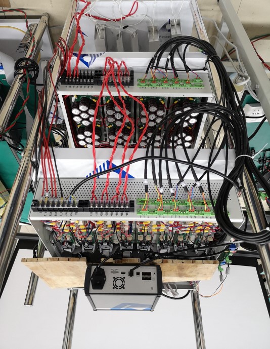
To verify the effectiveness and robustness of the proposed diagnostic method, a physical test platform for the cascaded H-bridge multilevel converter was built to evaluate its diagnostic performance. The experimental platform structure is shown in Figure 14, consisting of a PLECS RT-box controller, a control box, and a power supply box. The traditional dual-loop control scheme and the fault diagnosis algorithm are implemented in the RT-box controller, where both the sampling frequency and control frequency are set to 20 kHz to achieve satisfactory performance in dynamic response and diagnostic algorithm implementation. The control box is the main circuit for signal acquisition and switch control, including the sampling circuit, drive circuit, and cascaded H-bridge circuit. The power supply box contains the grid-side inductor, DC-link capacitors, and relays for switching power and load and bypassing H-bridges. Simulation and experimental parameters are listed in Table II. Open-circuit faults are simulated by disabling the drive signals of the switches.
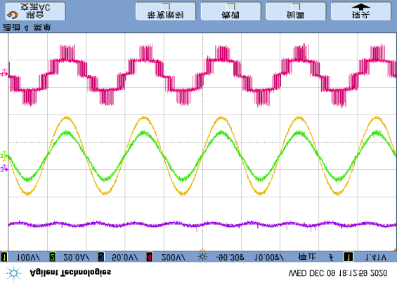
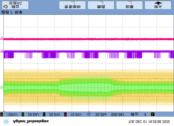
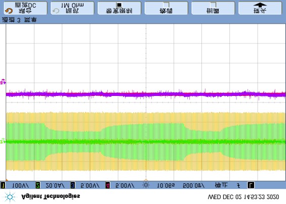
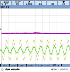
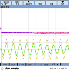
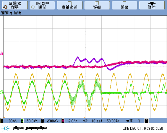
First, under normal conditions, the system achieves phase alignment between the grid voltage and grid current, and the DC-link voltage fluctuates around the reference value, as shown in Figure 15(a). After open-circuit faults occur in T12 and T22, Figure 15(b) shows distortions in both the grid current and DC-link voltage. To avoid severe DC voltage imbalance after the fault, all drive signals are blocked after two power frequency cycles to protect the system. Subsequently, the anti-interference performance of the proposed scheme was investigated.
A. Analysis of Anti-Interference Capability of the Proposed Method
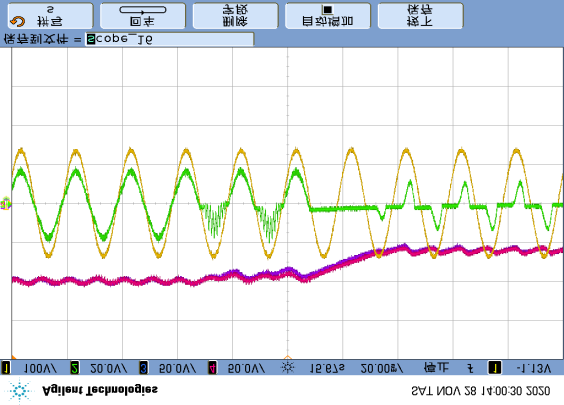
Regarding measurement noise, the sampling results in the RT-box controller are shown in Figure 16(a), where the AC signal is almost unaffected, but the sampled DC-link voltage contains obvious noise caused by electromagnetic interference and sampling. After applying the filtering method proposed in Figure 16(b), where g, a, and δ are set to 4100, 0.7, and 10Tc respectively, the measurement noise in the filtered voltage $u_{1f}$ is effectively suppressed.
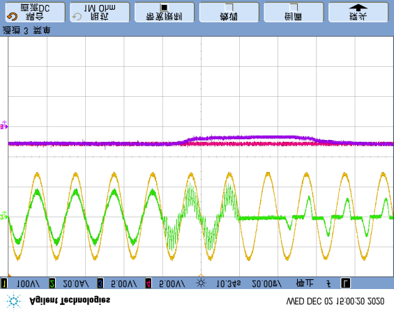
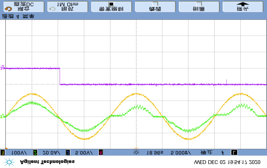
Table II Test Parameters of the Single-Phase CHBMC
| Parameter | Simulation Value | Experimental Value |
|---|---|---|
| Grid Voltage $u_N$ (RMS) | 4500 V | 100 V |
| Equivalent Filter Inductance $L_N$ | 10 mH | 3 mH |
| Parasitic Resistance $R_N$ | 0.02 Ω | 0.1 Ω |
| Reference DC-link Voltage $U_d$ | 3000 V | 100 V |
| DC-link Capacitance $C_i$ | 3.3 mF | 2.8 mF |
| Rated Equivalent Load $R_i$ | 20 Ω | 20 Ω |
| Number of Cascaded H-bridges $n$ | 3 | 2 |
| Switching Frequency $f_s$ | 500 Hz | 1000 Hz |
| Control Period $T_c$ | 50 µs | 50 µs |
| Grid Frequency $f_g$ | 50 Hz | 50 Hz |
| Detection Threshold $T_d$ | 0.7 | 0.7 |
| Diagnostic Threshold $T_{th}$ | 0.7 | 0.7 |
Due to the small time delay, the precision of output current calculation is improved. To further reduce the impact of continuous fluctuations in the filtered DC-link voltage on the calculation of voltage derivatives, $m$ of $u_i(k-m)$ is set to 2.
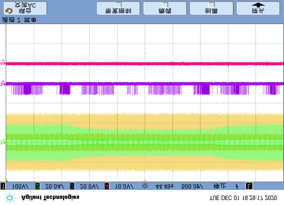
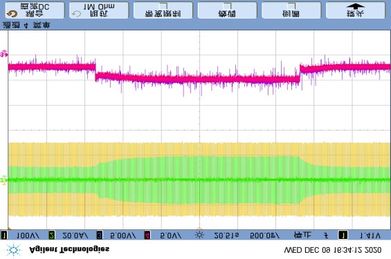
Since the proposed diagnostic method primarily relies on the DC-link voltage $u_i$ and grid current $i_N$ for fault calculations, any unexpected changes in these signals may lead to false fault detection. To analyze the anti-interference capability of the proposed method, a step change in $u_i$ between 85V and 100V was performed in Figure 17(a), causing the DC-link voltage to fluctuate up and down, and the grid current to decrease/increase accordingly. In Figure 17(b), the load power changed while the DC-link voltage remained constant, causing the grid current to vary with the load. In both cases, occasional single false alarms occurred, but three consecutive detections never happened. After setting the threshold $k_d$ to 3, false output of the detection feature $F_d$ will never occur.
Additionally, the performance of parameter/signal estimation was evaluated. Regarding fault detection, mismatches between the expected and actual values of $R_N$ and $L_N$ may affect detection accuracy. In experimental tests, the actual values of $R_N$ and $L_N$ were measured using a digital bridge, and the given values in the detection algorithm were altered to simulate the impact of parameter changes. Assuming $R_{N0}$ and $L_{N0}$ are the given values in the diagnostic algorithm, the changes in the detection variable $\varepsilon_d$ under different ratios of actual to given values are shown in Figure 18, where $\varepsilon_d$ takes its maximum value for 3 control cycles under normal conditions, or its minimum value for 3 control cycles under fault conditions. Regardless of normal or fault conditions, changes in $R_N$ have little effect on the detection variable, while the impact of $L_N$ is relatively significant.
 step change of $u_i$ between 85V and 100V; (b) step change of load between half-load (50%) and full-load (100%).)
The detection threshold $T_d$ is set to 0.7, which avoids false detection even under large parameter variations. Therefore, inductance estimation is not introduced.
In fault localization, the estimation methods for load current and capacitor primarily rely on the DC-link voltage $u_i$ and grid current $i_N$. Based on the trade-off between tracking speed and estimation accuracy, [h1 h2] is set to [0.2 -0.56] and μ is set to 1.1×10⁻⁴. In Figure 19, the load power changes while the DC-link voltage remains constant, causing the grid current to vary with the load. As shown in Figure 19(a), the estimated load current $i_{o1e}$ can accurately track the actual load current $i_{o1r}$. Even during transient changes, the estimate can track the true value within 1/2 line cycle. For capacitance estimation in Figure 19(b), where $C_{1e}$ is the estimated value and $C_{1r}$ is the reference value, the error between the estimated and reference values is very small even under transient changes.
However, when current distortion occurs, the actual system’s switching function is not equal to the switching function of the estimation algorithm, leading to reduced estimation accuracy.
From the experimental results in Figure 20, due to the delay in voltage change and the iterative control of the estimation algorithm, the estimates start to significantly deviate from the actual values after at least 1/4 line cycle. During this period, the fault detection variable has already detected the fault occurrence. Therefore, to minimize the impact of the fault on estimation accuracy, once the fault detection feature $F_d$ jumps to 1, the estimated load current and capacitance values are latched and remain unchanged throughout the diagnosis process.
Since faults may occur at any moment within a fundamental cycle, the diagnosis time may vary for different fault locations. Therefore, in this paper, the diagnosis time is defined as the time from the beginning of grid current distortion to the moment when all fault characteristics have appeared, specifically defined as:
$$
t_d = t_{sign} - t_{dist}
\tag{28}
$$
where $t_{sign}$ is the time when the last fault characteristic changes, and $t_{dist}$ is the time when the grid current begins to distort. Subsequently, the grid voltage, grid current, and fault trigger $F_t$ are displayed on the oscilloscope, while the real-time values of the detection variables and diagnostic features are acquired by the RT-box controller. In diagnostic comparison, 5% of ˂|iN|> is set as the variable judgment value, and the counter threshold $f_d$ is set to 3 to avoid misdiagnosis under extremely low current conditions.
B. Single Open-Circuit Fault Scenario
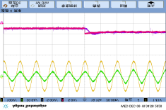
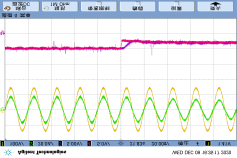
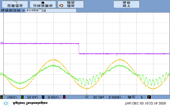
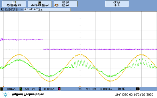
As shown in Figure 21(a), the fault trigger occurs during the positive half-cycle of $i_N$, but since T14 only operates when $i_N < 0$, current distortion appears at $t_s$. Since the fault characteristics of the detection and diagnostic variables do not immediately manifest, the diagnostic method cannot detect current residuals less than 5% ˂|iN|> and extremely low currents. When $\varepsilon_d$ and $G_{14}$ exceed the thresholds, and both $f_{c_14} \geq f_d$ and $k_{count} \geq k_d$ are satisfied simultaneously, the fault feature $F_{14}$ indicates that the faulty switch T14 has been identified. Fault detection and localization are completed at $t_1$, and the diagnosis time $t_d$ is 2.43 ms. When the T23 fault is triggered exactly within the operating cycle in Figure 21(b), current distortion occurs, and the fault characteristics of the detection variable $\varepsilon_d$ and diagnostic variable $G_{23}$ appear at $t_0$. Due to filtering delay and noise effects, the three consecutive fault events of $\varepsilon_d$ and $G_{23}$ do not simultaneously appear until $t_1$. Nevertheless, the diagnostic accuracy is well guaranteed, and the diagnosis time of 1.06 ms is also very short.
C. Multiple Open-Circuit Faults within a Single Unit
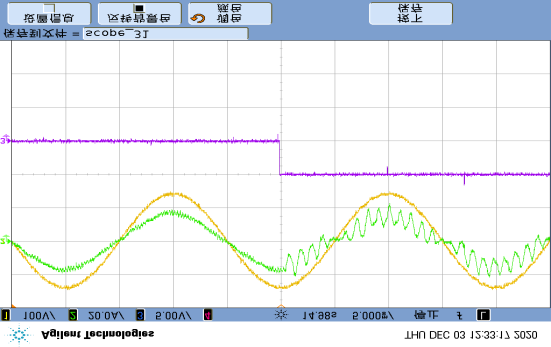
Figure 22 shows the test results of simultaneous multiple open-circuit faults in Unit 1. When T11 and T14 open-circuit faults are triggered during the positive half-cycle of $i_N$ in Figure 22(a),
 to full-load (100%).)
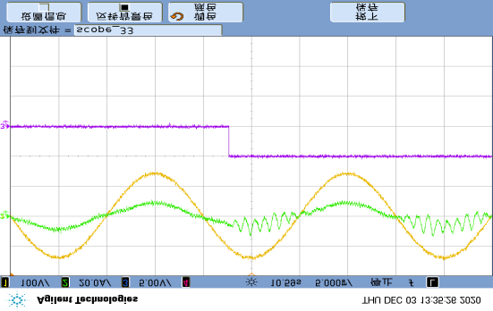
current distortion occurs at $t_s$. Due to the extremely low grid current and residual less than 5% ˂|iN|>, the fault characteristics of the diagnostic variables do not immediately appear. At time $t_1$, three consecutive fault events of the detection variable $\varepsilon_d$ and diagnostic variable $G_{14}$ occur. Afterwards, at $t_2$, the identification of the T11 fault is achieved, limiting the entire localization time to $t_d = 4.71$ ms. In Figure 22(b), T11 and T12 open-circuit faults are introduced, affecting the entire current path. Starting from current distortion at $t_s$, T12 is first located as the faulty switch after 1.84 ms, and the location characteristic of T11 is not demonstrated until $t_2$. Despite the influence of current residual and detection variables by noise, both switches are effectively identified within $t_d = 7.29$ ms.
D. Multiple Open-Circuit Faults in Multiple Units
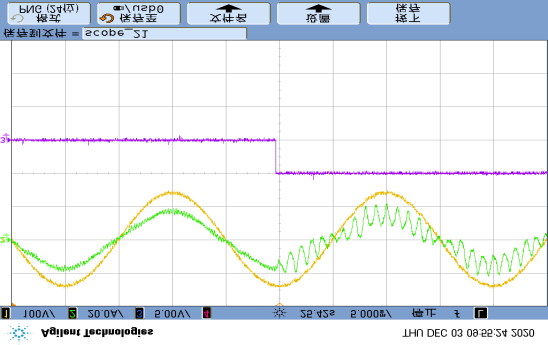
To analyze the diagnostic performance of multiple open-circuit faults in various cells, two faults occur simultaneously at T11 in Unit 1 and T21 in Unit 2, which only affect the negative half-cycle of $i_N$. Current distortion occurs at $t_s$ in Figure 23(a). The diagnostic condition is not met until $t_1$, when T21 is identified as the faulty switch. Afterwards, at $t_2$, the open-circuit of T11 is identified, completing the entire localization time limited to 5.42 ms. Regarding the impact of T14 and T22 open-circuit faults on the entire cycle of $i_N$ in Figure 23(b), the T22 fault is located within 1.57 ms because the current distortion only occurs in its own positive half-cycle of $i_N$. Due to the open-circuit fault of T14 being detected only in the negative cycle, the fault localization of T14 is not completed until $t_2$, with a diagnosis time of 7.28 ms.
E. Diagnostic Results under Light-Load Conditions
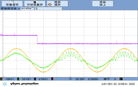
To demonstrate diagnostic performance under light-load conditions, Figure 24 presents experimental results for single and multiple faults. In Figure 24(a), current distortion caused by the T12 fault appears at $t_0$. Subsequently, continuous fault characteristics are detected for the first time at $t_1$, taking approximately 1.21 ms, and are not affected by the light-load condition. Next, in Figure 24(b), T12 and T24 open-circuit faults affecting the entire current cycle are considered. Since current distortion only occurs in its own positive half-cycle of $i_N$, T12 is identified as the faulty switch within 0.33 ms. Affected by low current and noise, the fault localization of T24 is not completed until $t_2$, with the entire diagnosis time being 9.57 ms, less than 1/2 line cycle. Although the dual effects of low current and measurement noise may prolong the diagnosis time, the diagnosis process can still be completed within one power frequency cycle, demonstrating the good robustness and diagnostic performance of the proposed algorithm.
F. Comparison with Related Methods
From the above experimental results, it can be seen that the diagnosis time for single-switch faults and simultaneous multiple faults affecting only half of the grid current cycle is about 1/4 of a power frequency cycle, while other multiple fault diagnosis processes can be completed within less than one grid cycle considering different fault trigger times. Since different authors verify the diagnostic performance of the proposed algorithm under different control frequencies, switching frequencies, and numbers of H-bridge cells, the system’s power frequency cycle is chosen as the reference for diagnosis time to analyze and compare the diagnostic performance of various algorithms. This diagnosis time statistics do not include the time when the switch fault occurs but is not activated, as shown in Table III.
Based on the classification of computational burden, the computational burden of the proposed method based on residual calculation and comparison is moderate. Compared with the diagnostic methods in [28],[29], this method can achieve detection and localization of multiple faults by using simple estimation models and diagnostic variables, thereby expanding the application range of the diagnostic algorithm. Compared with [31], the proposed method does not require the relatively complex matrix updates for fault localization and can be simply realized by comparing individual diagnostic variables and counters. Additionally, the impact of large parameter changes and measurement noise on the diagnostic algorithm is analyzed. Online parameter estimation based on RLS, noise filters, and additional detection algorithms are introduced to enhance the robustness and accuracy of the diagnostic method under various extreme conditions.
G. Further Discussion of the Proposed Method
Regarding threshold selection in detection and localization, the settings of the diagnostic threshold $T_{th}$, detection threshold $T_d$, and count thresholds $f_d$ and $k_d$ depend on the influence degree of various operating conditions, parameter inaccuracies, and measurement noise. Based on the evolution of hardware system influences, these thresholds can be adjusted to strike a compromise between diagnosis time and diagnosis accuracy. The size of measurement noise is directly related to hardware circuit design, sensor sampling accuracy, and operating environment. In practical applications, the decision to add extra filtering or detection algorithms to the diagnostic method can be made based on the degree of measurement noise impact. Meanwhile, online estimation of capacitor and inductor parameters can be added to improve the reliability of the algorithm during long-term operation.
Table III Comparison of the Proposed Method with Related Methods
| Algorithm | Required Sensors | Single-Switch Fault Diagnosis Time | Multi-Switch Fault Diagnosis Time | Diagnosis Level | Method Used | Computational Burden |
|---|---|---|---|---|---|---|
| [20] | Control System | < 3 line cycles | Impossible | Cell and Switch | Slope Calculation and Comparison | Moderate |
| [21] | Additional Voltage Sensors | < 1 line cycle | Impossible | Cell | DFT and Comparison | High |
| [22] | Additional Voltage Sensors | < 3 line cycles | < 7 line cycles | Cell and Switch | FFT and Principal Component Analysis | High |
| [23] | Additional Voltage Sensors | < 1 line cycle | Impossible | Cell | Two Comparisons | Low |
| [24] | Additional Voltage Sensors | < 1/4 line cycle | < 1 line cycle | Cell | Two Comparisons | Low |
| [28] | Control System | < 1/2 line cycle | < 1/2 line cycle | Cell and Switch Pair | Residual Calculation and Comparison | Moderate |
| [29] | Control System | < 1/4 line cycle | Impossible | Cell and Switch | Residual Calculation and Comparison | Moderate |
| [31] | Control System | < 1/4 line cycle | < 1 line cycle | Cell and Switch | Residual Calculation and Fault Location Matrix | Moderate |
| Proposed Method | Control System | < 1/4 line cycle | < 1 line cycle | Cell and Switch | Residual Calculation and Comparison | Moderate |
VI. CONCLUSION
This paper proposes a fast open-circuit fault diagnosis scheme for cascaded H-bridge multilevel converters to detect and locate single or multiple switch faults. The output current of each H-bridge is selected as the diagnostic signal, whose actual and expected values are obtained from the main circuit and control system without requiring additional sensors. Combining residual analysis and various operating conditions, normalized diagnostic variables and diagnostic counters are designed to identify faults. Furthermore, by introducing noise filters, parameter estimation, and enhanced detection methods, the diagnostic method becomes insensitive to large parameter changes and measurement noise, suitable for circuit systems under long-term operation. Experimental results show that the proposed method is effective and robust under different fault scenarios and operating conditions. The advantage of this method lies in being able to locate single and multiple faults within less than one grid cycle using only two normalized thresholds and two comparison counters, regardless of the number of faulty switches and faulty cells. Meanwhile, the diagnostic variables correspond directly to the switches of each H-bridge, making it easy to extend to cascaded H-bridge multilevel converters with an arbitrary number of submodules. However, when the load is too light, fault characteristics may be overwhelmed by noise, failing to satisfy the counter’s diagnostic conditions, resulting in undiagnosed faults, which will be further studied in future work.


 1314
1314

 被折叠的 条评论
为什么被折叠?
被折叠的 条评论
为什么被折叠?
 到【灌水乐园】发言


