NCCL的Double Binary Tree实现原理

假设每个节点上的数据Size是S，单向带宽为B；Node to Node传输1个byte的延迟为L；

无脑单二叉树，使用流式加和和传输，汇总到root，总消耗时间为: 2*S/B + lgN*L；其中，2*S为每个非叶子节点需要接收的数据量，瓶颈在此；root再广播到所有节点，消耗同样时间；因此，AllReduce总耗时为2*(2*S/B + lgN*L);

RingAllReduce：(2*S*(N-1)/B/N + 2*(N-1)*L)

double binary tree延迟小的原因：hop次数是lgN（RingAllReduce是N-1)

吞吐量高的原因：每个节点，把数据流动起来了，子节点传过来一部分，加和这部分，传出给父节点；

第1个tree，所有节点只传输和加和前一半数组；第2个tree，只做后一半数组；

假设每个节点上的数据Size是S，单向带宽为B；延迟是lgN*单跳延迟L，下面先不考虑延迟；

第1个tree，每个节点的发射耗时是(S/2)/B，每个叶子节点的接收耗时为0，每个非叶子节点的接收耗时为S/B，总共S/B的耗时可以将这前一半数据流式汇总到root节点；第2个tree，数字也是这样，S/B的耗时将后一半数据流式汇总到root节点；2个Tree同时开工，所有节点的发送带宽和接收带宽都打满了（因为每个节点既是另2个节点的father，也是另2个节点的child），S/B的耗时将数据汇总到2个root节点；

Broadcast过程，雷同，从上往下传输，还是2个Tree同时开工，S/B的耗时将结果广播至所有节点；

因此，double binary tree的AllReduce总耗时是2*S/B；

再加上延迟，就是(2*S/B + lgN*L);

比AllReduce的(2*S*(N-1)/B/N + 2*(N-1)*L)，在L项上少一半个数量级；

RingAllReduce，每次每个节点等量的发送和接收，所以接收到的加和完后，没有带宽再同时发送了！

Massively Scale Your Deep Learning Training with NCCL 2.4

By Sylvain Jeaugey

Imagine using tens of thousands of GPUs to train your neural network. Using multiple GPUs to train neural networks has become quite common with all deep learning frameworks, providing optimized, multi-GPU, and multi-machine training. Allreduce operations, used to sum gradients over multiple GPUs, have usually been implemented using rings [1] [2] to achieve full bandwidth. The downside of rings is that latency scales linearly with the number of GPUs, preventing scaling above hundreds of GPUs. Enter NCCL 2.4.

Many large scale experiments have replaced the flat ring by a hierarchical, 2D ring algorithm [3] [4] [5] to get reasonably good bandwidth while lowering latency.

NCCL 2.4 now adds double binary trees, which offer full bandwidth and a logarithmic latency even lower than 2D ring latency.

Double binary trees

Double binary trees were introduced in MPI in 2009 [6] and offer the advantage of combining both full bandwidth for broadcast and reduce operations (which can be combined into an allreduce performing a reduce, then a broadcast) and a logarithmic latency, enabling good performance on small and medium size operations.

In NCCL, we build binary trees using an easy-to-implement pattern which maximizes locality, as shown in figure 1.

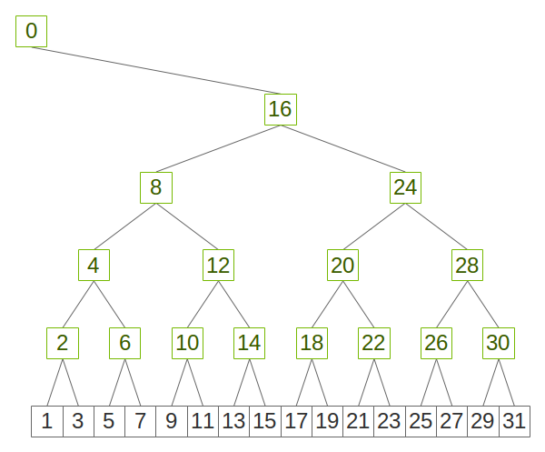
Figure 1. Binary tree using a power-of-two pattern

Double binary trees rely on the fact that half or less ranks in a binary tree are nodes and half (or more) ranks are leaves. Therefore, we can build a second tree using leaves as nodes and vice-versa for each binary tree. There might be one rank which is a leaf on both trees but no rank is a node on both trees.

Figure 2 shows how we can use the pattern above to build a double binary tree by flipping the tree to invert nodes and leaves.

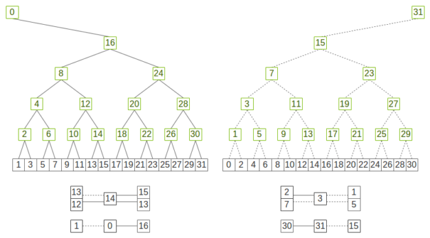
Figure 2. Two complementary binary trees where each rank is at most a node in one tree and a leaf in the other.

If you superimpose the two trees, all ranks have both two parents and two children except for the root ranks, which only have one parent and one child. If we use each of the two trees to process half of the data, each rank will at most receive half of the data twice and send half of the data twice, which is as optimal as rings in terms of data sent/received.

Performance at scale

We tested NCCL 2.4 on various large machines, including the Summit [7] supercomputer, up to 24,576 GPUs. As figure 3 shows, latency improves significantly using trees. The difference from ring increases with the scale, with up to 180x improvement at 24k GPUs.

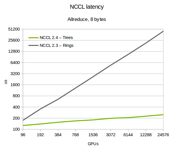
Figure 3. NCCL latency on up to 24,576 GPUs

We confirmed that the system maintains full bandwidth with double binary trees. At scale, bandwidth degrades a bit when we cross L3 switches in the InfiniBand fabric, which we believe is due to inefficiencies between the NCCL communication pattern and InfiniBand routing algorithms.

While not perfect, this might be improved in the future. Even so, trees still show a clear advantage even when limited in bandwidth because of their small initial latency. However, NCCL automatically switches back to rings when that pattern results in greater bandwidth.

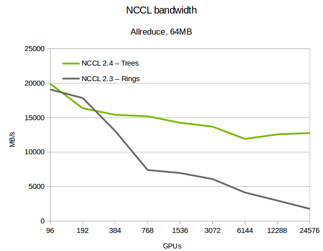
Figure 4. NCCL bus bandwidth on up to 24,576 GPUs

Effect on DL training

Figure 5 shows performance improvement on DL training is significant, and increases as we scale to larger numbers of GPUs.

We compared NCCL 2.3 and NCCL 2.4, as well as the 2D hierarchical rings using NCCL 2.3. The hierarchical ring is a 2D ring (intra-node/inter-node being the 2 dimensions) which performs a reduce-scatter operation inside the node, then multiple all-reduce operations between nodes, then an all-gather operation inside the node again.

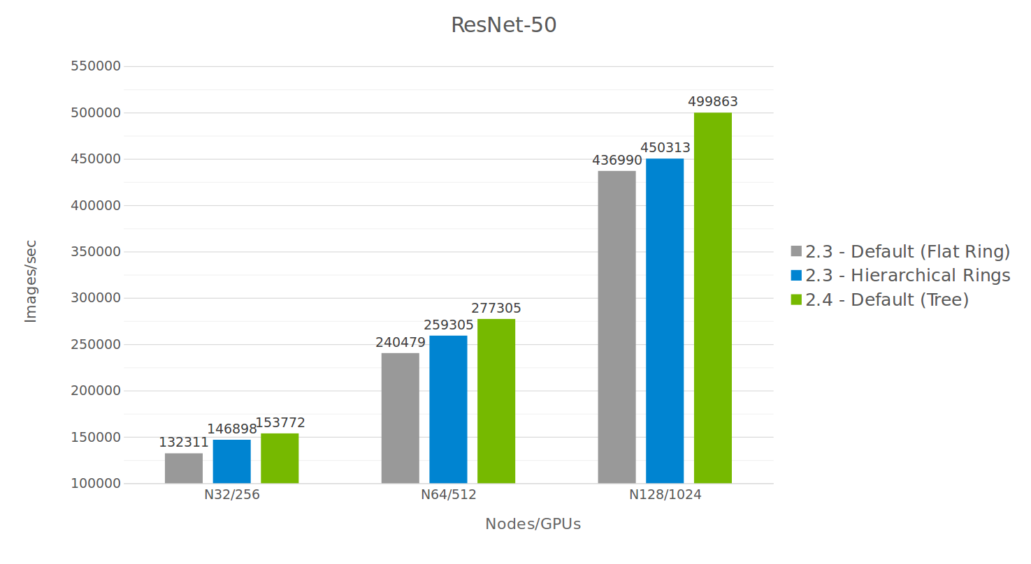
Fig 5. Performance comparison on ResNet50

While the hierarchical rings perform better than non-hierarchical rings, their advantage at scale remains constant. The tree algorithm, on the other hand, offers an increasing advantage as we scale.

Other features

Network error handling

NCCL operations behave as CUDA kernels. Once the operation launches on a CUDA stream, the user waits for its completion using stream semantics, e.g. cudaStreamQuery or cudaStreamSynchronize. It’s convenient to have the NCCL operation start as soon as the CUDA kernel producing the data completes, but it doesn’t let NCCL report errors during communication.

However, as we start using the network between nodes, network errors can occur and could prevent the NCCL operation from completing, causing a hang. This becomes increasingly important as we grow in size. NCCL 2.4 introduces two new verbs : ncclCommGetAsyncError and ncclCommAbort to handle this.

Programs can call ncclCommGetAsyncError in a loop waiting for operations to complete. If an error happens, they can abort the application or try to only abort the communicator operation with ncclCommAbort, then recreate a new communicator with the remaining nodes.

An example of using those two functions can be found in the documentation. Here is a simplified example illustrating the usage of those two functions :

int ncclStreamSynchronize(cudaStream_t stream, ncclComm_t comm) {
   while (1) {
      cudaError_t cudaErr = cudaStreamQuery(stream);
      ncclResult_t ncclAsyncErr, ncclErr;
      ncclErr = ncclCommGetAsyncError(comm, &ncclAsyncErr);

      if (cudaErr == cudaSuccess) return 0;
      if (cudaErr != cudaErrorNotReady || ncclErr != ncclSuccess) {
         printf("CUDA/NCCL Error : %d/%d\n", cudaErr, ncclErr);
         return 1; // Abnormal error
      }
            if (ncclAsyncErr != ncclSuccess) { // Async network error
               // Stop and destroy communicator 
              if (ncclCommAbort(comm) != ncclSuccess) {
                 printf("NCCL Comm Abort error : %d\n", ncclErr);          
                 return 1; // Abnormal error
              }
             return 2; // Normal error : may recreate a new comm
          }
       }
    }

This function can be generalized to including polling for other asynchronous operations, such as MPI, socket, or other I/O operations.

Support for more networks

NCCL 2.4 comes with native support for TCP/IP Sockets and InfiniBand Verbs. TCP/IP sockets should work on most networks but can also be bandwidth- and latency-limited due to limitations in the kernel driver. CPU affinity can also be complex to handle.

The InfiniBand verbs library enables an application to bypass the kernel and directly handle all network communication from user space. This is the prefered API to use on InfiniBand and RDMA over Converged Ethernet (RoCE) capable hardware..

Some other networking providers have different network APIs which provides better performance than TCP/IP sockets. Those vendors can get the best performance from NCCL by implementing an external network plugin to be used by NCCL when present. This can be provided in the form of a library named libnccl-net.so. NCCL includes an example in ext-net/dummy. Check out one example in the plugin for the libfabrics API.

Get NCCL 2.4 Today

You can get started scaling your applications to massive numbers of GPUs today. Pre-built NCCL package can be obtained from the download page. The source code is also available on github.

References

[1] Baidu Allreduce

[2] Horovod

[3] Xianyan Jia, Shutao Song, Wei He, Yangzihao Wang, Haidong Rong, Feihu Zhou, Liqiang Xie, Zhenyu Guo, Yuanzhou Yang, Liwei Yu, Tiegang Chen, Guangxiao Hu, Shaohuai Shi, Xiaowen Chu; Highly Scalable Deep Learning Training System with Mixed-Precision: Training ImageNet in Four Minutes

[4] Hiroaki Mikami, Hisahiro Suganuma, Pongsakorn U-chupala, Yoshiki Tanaka, Yuichi Kageyama; ImageNet/ResNet-50 Training in 224 Seconds

[5] Chris Ying, Sameer Kumar, Dehao Chen, Tao Wang, Youlong Cheng; Image Classification at Supercomputer Scale

[6] Peter Sanders; Jochen Speck, Jesper Larsson Träff (2009); Two-tree algorithms for full bandwidth broadcast, reduction and scan

[7] Summit Supercomputer