


目录
1. 模型简介
1.1 用途
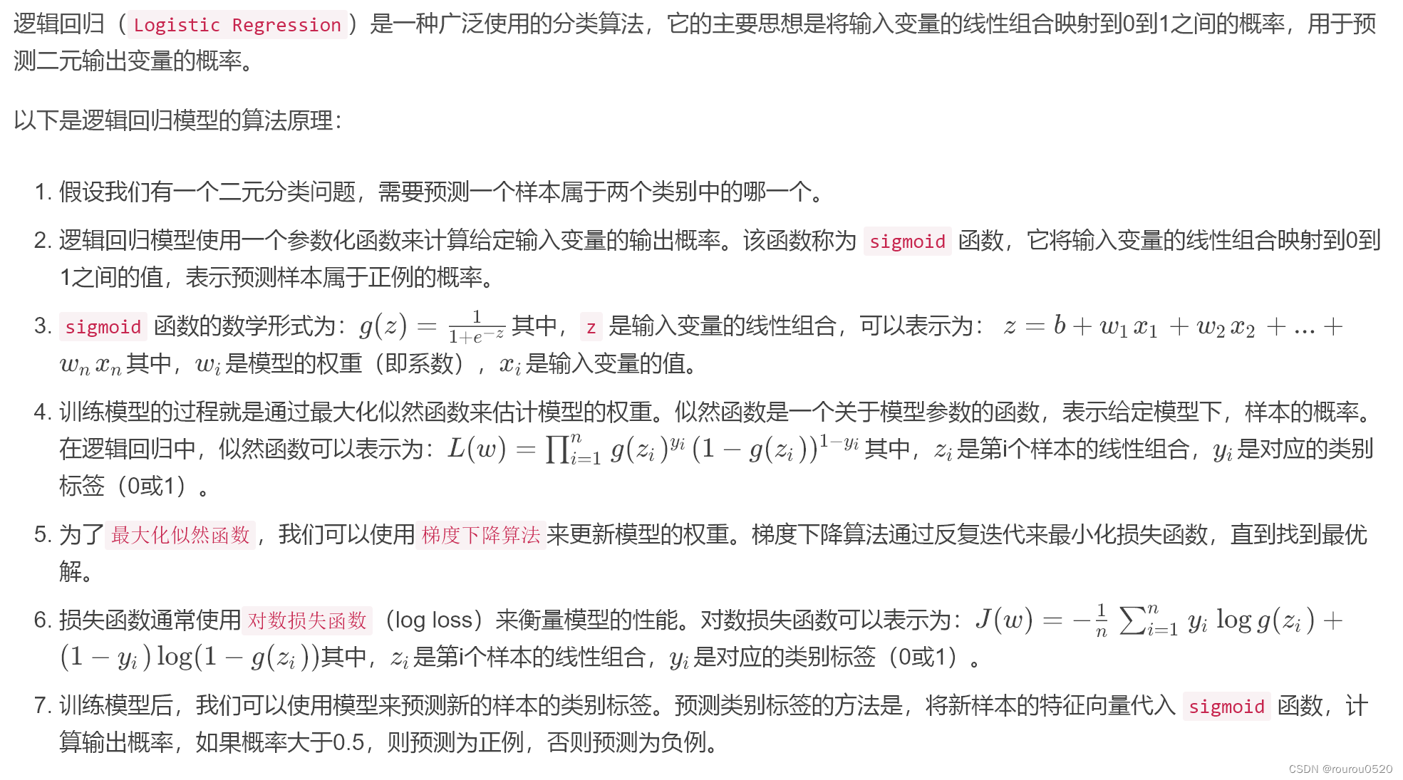
逻辑回归是线性分类器(线性模型)—— 主要用于二分类问题
注意:逻辑回归虽然名字中有回归二字,但是它不是回归算法,而是分类算法。
1.2 逻辑回归问题解决的常规步骤
原文链接:https://blog.youkuaiyun.com/m0_47256162/article/details/129776507?ops_request_misc=%257B%2522request%255Fid%2522%253A%2522169174457516800182184745%2522%252C%2522scm%2522%253A%252220140713.130102334…%2522%257D&request_id=169174457516800182184745&biz_id=0&utm_medium=distribute.pc_search_result.none-task-blog-2alltop_positive~default-3-129776507-null-null.142v92controlT0_2&utm_term=%E9%80%BB%E8%BE%91%E5%9B%9E%E5%BD%92python%E4%BB%A3%E7%A0%81%E5%AE%9E%E7%8E%B0&spm=1018.2226.3001.4187
2. python实现二分类逻辑回归
multiregression文件
2.1 使用函数model = LogisticRegression()
from sklearn.datasets import load_breast_cancer
import pandas as pd
from sklearn.model_selection import train_test_split
from sklearn.linear_model import LogisticRegression
from sklearn.metrics import classification_report
import warnings
import sklearn.metrics as sm #生成混淆矩阵的库
import seaborn as sn  #混淆矩阵可视化的库
import matplotlib.pyplot as plt #画图
warnings.filterwarnings('ignore')

cancer = load_breast_cancer()
data = cancer["data"]
col = cancer['feature_names']
x = pd.DataFrame(data, columns=col)
target = cancer.target.astype(int)
y = pd.DataFrame(target, columns=['target'])
x_train, x_test, y_train, y_test = train_test_split(x, y, test_size=0.3, random_state=1)
model = LogisticRegression()   #默认参数
model.fit(x_train, y_train)     #模型训练
y_pred = model.predict(x_test)     #模型预测
print(classification_report(y_test, y_pred))   #评估报告
m = sm.confusion_matrix(y_test, y_pred) #生成混淆矩阵
print('混淆矩阵为:', m, sep='\n')
ax = sn.heatmap(m, annot=True, fmt='.20g')
ax.set_title('confusion matrix')
ax.set_xlabel('predict')
ax.set_ylabel('true')
plt.show() #混淆矩阵可视化
注: LogisticRegression() 函数参数的说明:
PS:但是没见人用过超参数调优或者其他方法来调节参数
(1)penalty: 表示惩罚项(正则化类型)。字符串类型,取值为’l1’ 或者 ‘l2’,默认为’l2’。
l1:向量中各元素绝对值的和,作用是产生少量的特征,而其他特征都是0,常用于特征选择;
l2:向量中各个元素平方之和,作用是选择较多的特征,使他们都趋近于0。
注意:如果模型的特征非常多,我们想要让一些不重要的特征系数归零,从而让模型系数稀疏化的话,可以使用l1正则化。
(2)tol: 浮点型,默认为1e-4;表示迭代终止判断的误差范围
(3)C: 浮点型(为正的浮点数),默认为1.0;表示正则化强度的倒数(目标函数约束条件)。数值越小表示正则化越强。
(4)solver: 用于优化问题的算法。取值有{‘newton-cg’, ‘lbfgs’, ‘liblinear’, ‘sag’, ‘saga’},默认为’liblinear’;
对于小数据集来说,“liblinear”就够了,而“sag”和’saga’对于大型数据集会更快。
对于多类问题,只有’newton-cg’, ‘sag’, ‘saga’和’lbfgs’可以处理多项损失;“liblinear”仅限于一对一分类。
注意:上面的penalty参数的选择会影响参数solver的选择。如果是l2正则化,那么4种算法{‘newton-cg’, ‘lbfgs’, ‘liblinear’, ‘sag’}都可以选择。但如果penalty是l1正则化的话,就只能选择‘liblinear’了。这是因为L1正则化的损失函数不是连续可导的,而{‘newton-cg’, ‘lbfgs’,‘sag’}这三种优化算法时都需要损失函数的一阶或者二阶连续导数。而‘liblinear’并没有这个依赖。
(5)multi_class: 字符串类型,取值有{ovr’, ‘multinomial’},默认为’ovr’;
如果选择的选项是“ovr”,那么则为“one-versus-rest(OvR)”分类。multinomial则为“many-vs-many(MvM)”分类。
“one-versus-rest(OvR)”分类:无论你是多少元的逻辑回归,都可以看做多个二元逻辑回归的组合。具体做法是:对于第K类的分类决策,我们把所有第K类的样本作为正例,除了第K类样本以外的所有样本都作为负例,然后在上面做二元逻辑回归,得到第K类的分类模型。其他类的分类模型获得以此类推。
“many-vs-many(MvM)”分类:如果模型有T类,我们每次在所有的T类样本里面选择两类样本出来,不妨记为T1类和T2类,把所有的输出为T1和T2的样本放在一起,把T1作为正例,T2作为负例,进行二元逻辑回归,得到模型参数。我们一共需要T(T-1)/2次分类(即组合数)。
(6)n_jobs:整数类型,默认是1;
如果multi_class=‘ovr’ ,则为在类上并行时使用的CPU核数。无论是否指定了multi_class,当将
’ solver ’设置为’liblinear’时,将忽略此参数。如果给定值为-1,则使用所有核。
2.2 自定义函数(有可视化边界图展现regression2)
import numpy as np
import matplotlib.pyplot as plt
from sklearn.datasets import load_iris
from sklearn.model_selection import train_test_split

# 设置随机种子
seed_value = 2023
np.random.seed(seed_value)

# Sigmoid激活函数
def sigmoid(z):
    return 1 / (1 + np.exp(-z))

# 定义逻辑回归算法
class LogisticRegression:
    def __init__(self, learning_rate=0.003, iterations=100):
        self.learning_rate = learning_rate  # 学习率
        self.iterations = iterations  # 迭代次数

    def fit(self, X, y):
        # 初始化参数
        self.weights = np.random.randn(X.shape[1])
        self.bias = 0

        # 梯度下降
        for i in range(self.iterations):
            # 计算sigmoid函数的预测值, y_hat = w * x + b
            y_hat = sigmoid(np.dot(X, self.weights) + self.bias)

            # 计算损失函数
            loss = (-1 / len(X)) * np.sum(y * np.log(y_hat) + (1 - y) * np.log(1 - y_hat))

            # 计算梯度
            dw = (1 / len(X)) * np.dot(X.T, (y_hat - y))
            db = (1 / len(X)) * np.sum(y_hat - y)

            # 更新参数
            self.weights -= self.learning_rate * dw
            self.bias -= self.learning_rate * db

            # 打印损失函数值
            if i % 10 == 0:
                print(f"Loss after iteration {i}: {loss}")

    # 预测
    def predict(self, X):
        y_hat = sigmoid(np.dot(X, self.weights) + self.bias)
        y_hat[y_hat >= 0.5] = 1
        y_hat[y_hat < 0.5] = 0
        return y_hat

    # 精度
    def score(self, y_pred, y):
        accuracy = (y_pred == y).sum() / len(y)
        return accuracy


# 导入数据
iris = load_iris()
X = iris.data[:, :2]
y = (iris.target != 0) * 1

# 划分训练集、测试集
X_train, X_test, y_train, y_test = train_test_split(X, y, test_size=0.15, random_state=seed_value)

# 训练模型
model = LogisticRegression(learning_rate=0.03, iterations=1000)
model.fit(X_train, y_train)

# 结果
y_train_pred = model.predict(X_train)
y_test_pred = model.predict(X_test)

score_train = model.score(y_train_pred, y_train)
score_test = model.score(y_test_pred, y_test)

print('训练集Accuracy: ', score_train)
print('测试集Accuracy: ', score_test)

# 可视化决策边界
x1_min, x1_max = X[:, 0].min() - 0.5, X[:, 0].max() + 0.5
x2_min, x2_max = X[:, 1].min() - 0.5, X[:, 1].max() + 0.5
xx1, xx2 = np.meshgrid(np.linspace(x1_min, x1_max, 100), np.linspace(x2_min, x2_max, 100))
Z = model.predict(np.c_[xx1.ravel(), xx2.ravel()])
Z = Z.reshape(xx1.shape)
plt.contourf(xx1, xx2, Z, cmap=plt.cm.Spectral)
plt.scatter(X[:, 0], X[:, 1], c=y, cmap=plt.cm.Spectral)
plt.xlabel("Sepal length")
plt.ylabel("Sepal width")
plt.show()
3. python实现多分类逻辑回归
3.1 理论实现的方法:
方式一:修改逻辑回归的损失函数,使用softmax函数构造模型解决多分类问题,softmax分类模型会有相同于类别数的输出,输出的值为对于样本属于各个类别的概率,最后对于样本进行预测的类型为概率值最高的那个类别。
方式二:根据每个类别都建立一个二分类器,本类别的样本标签定义为0,其它分类样本标签定义为1,则有多少个类别就构造多少个逻辑回归分类器
若所有类别之间有明显的互斥则使用softmax分类器,若所有类别不互斥有交叉的情况则构造相应类别个数的逻辑回归分类器。
3.2 多分类softmax回归原理参考一下内容
参考https://www.zhihu.com/question/23765351/answer/98897364
原文链接:https://blog.youkuaiyun.com/qq_52358603/article/details/127511045
3.3 python代码
multireg2代码文件
3.3.1 通过函数实现
sklearn中LogisticsRegression类中,参数multi_class设置为multinomial时,使用的就是softmax回归
from sklearn import datasets #导入数据集模块
from sklearn.model_selection import train_test_split #数据集划分
from sklearn.linear_model import LogisticRegression
from sklearn.metrics import classification_report   #用于显示主要分类指标的文本报告
import sklearn.metrics as sm #生成混淆矩阵的库
import seaborn as sn  #混淆矩阵可视化的库
import matplotlib.pyplot as plt #画图
import numpy as np
from sklearn.model_selection import GridSearchCV
#--------------------------------1.加载数据集---------------------------------#
iris = datasets.load_iris()#加载鸢尾花数据集
print(iris)
X = iris.data #输入特征
Y = iris.target #标签(输出特征)
print(X)
print('----------------')
print(Y)
print('----------------')
print('鸢尾花输入特征的维度是{}'.format(X.shape))
print('鸢尾花标签的维度是{}'.format(Y.shape))

#--------------------------------2.划分数据集---------------------------------#
X_train, X_test, Y_train, Y_test = train_test_split(X, Y, test_size=0.2, random_state=45) # 数据划分

#--------------------------------3.模型训练与预测---------------------------------#
#sklearn中LogisticsRegression类中,参数multi_class设置为multinomial时,使用的就是softmax回归
model2 = LogisticRegression(multi_class='multinomial')
model2.fit(X_train, Y_train)
# 评分
model2.score(X_train, Y_train)
model2.score(X_test, Y_test)
y_pred2 = model2.predict(X_test)     #模型预测

#--------------------------------4.模型评估---------------------------------#
m2 = sm.confusion_matrix(Y_test, y_pred2) #生成混淆矩阵
print('混淆矩阵为:', m2, sep='\n')
ax = sn.heatmap(m2, annot=True, fmt='.20g')
ax.set_title('confusion matrix')
ax.set_xlabel('predict')
ax.set_ylabel('true')
plt.show() #混淆矩阵可视化
print(classification_report(Y_test, y_pred2))   #评估报告
3.3.2 自定义函数实现
数据集和KNN那个博文用的是同样的数据集。
数据地址:https://github.com/WenDesi/lihang_book_algorithm/blob/master/data/train.csv
import math
import pandas as pd
import numpy as np
import random
import time

from sklearn.model_selection import train_test_split
from sklearn.metrics import accuracy_score


class Softmax(object):

    def __init__(self):
        self.learning_step = 0.000001           # 学习速率
        self.max_iteration = 100000             # 最大迭代次数
        self.weight_lambda = 0.01               # 衰退权重

    def cal_e(self,x,l):
        '''
        计算博客中的公式3
        '''

        theta_l = self.w[l]
        product = np.dot(theta_l,x)

        return math.exp(product)

    def cal_probability(self,x,j):
        '''
        计算博客中的公式2
        '''

        molecule = self.cal_e(x,j)
        denominator = sum([self.cal_e(x,i) for i in range(self.k)])

        return molecule/denominator


    def cal_partial_derivative(self,x,y,j):
        '''
        计算博客中的公式1
        '''

        first = int(y==j)                           # 计算示性函数
        second = self.cal_probability(x,j)          # 计算后面那个概率

        return -x*(first-second) + self.weight_lambda*self.w[j]

    def predict_(self, x):
        result = np.dot(self.w,x)
        row, column = result.shape

        # 找最大值所在的列
        _positon = np.argmax(result)
        m, n = divmod(_positon, column)

        return m

    def train(self, features, labels):
        self.k = len(set(labels))

        self.w = np.zeros((self.k,len(features[0])+1))
        time = 0

        while time < self.max_iteration:
            print('loop %d' % time)
            time += 1
            index = random.randint(0, len(labels) - 1)

            x = features[index]
            y = labels[index]

            x = list(x)
            x.append(1.0)
            x = np.array(x)

            derivatives = [self.cal_partial_derivative(x,y,j) for j in range(self.k)]

            for j in range(self.k):
                self.w[j] -= self.learning_step * derivatives[j]

    def predict(self,features):
        labels = []
        for feature in features:
            x = list(feature)
            x.append(1)

            x = np.matrix(x)
            x = np.transpose(x)

            labels.append(self.predict_(x))
        return labels


if __name__ == '__main__':

    print('Start read data')

    time_1 = time.time()

    raw_data = pd.read_csv('../data/train.csv', header=0)
    data = raw_data.values

    imgs = data[0::, 1::]
    labels = data[::, 0]

    # 选取 2/3 数据作为训练集, 1/3 数据作为测试集
    train_features, test_features, train_labels, test_labels = train_test_split(
        imgs, labels, test_size=0.33, random_state=23323)
    # print train_features.shape
    # print train_features.shape

    time_2 = time.time()
    print('read data cost '+ str(time_2 - time_1)+' second')

    print('Start training')
    p = Softmax()
    p.train(train_features, train_labels)

    time_3 = time.time()
    print('training cost '+ str(time_3 - time_2)+' second')

    print('Start predicting')
    test_predict = p.predict(test_features)
    time_4 = time.time()
    print('predicting cost ' + str(time_4 - time_3) +' second')

    score = accuracy_score(test_labels, test_predict)
    print("The accruacy socre is " + str(score))
此部分代码参考:
原文链接:https://blog.youkuaiyun.com/wds2006sdo/article/details/53699778
https://blog.youkuaiyun.com/qq_34695147/article/details/70663588
部分参考文章:
原文链接:https://blog.youkuaiyun.com/weixin_55073640/article/details/124683459


 被折叠的 条评论
为什么被折叠?
被折叠的 条评论
为什么被折叠?
 到【灌水乐园】发言


