BIM/I-FGSM对抗样本生成算法实现（pytorch版）

入梦风行

已于 2025-04-08 17:36:17 修改

阅读量892

点赞数 25

分类专栏：深度学习文章标签：算法 pytorch 人工智能 python 深度学习安全

于 2025-03-30 22:27:03 首次发布

本文链接：https://blog.youkuaiyun.com/qq_62107003/article/details/146778946

版权

深度学习专栏收录该内容

10 篇文章

订阅专栏

BIM/I-FGSM对抗样本生成算法

一、理论部分
- 1.1 核心思想
- 1.2 数学形式
- 1.3 BIM 的优缺点
- 1.4 BIM 与 FGSM、PGD 的关系
- 1.5 实际应用建议
二、代码实现
- 2.1 导包
- 2.2 数据加载和处理
- 2.3 网络构建
- 2.4 模型加载
- 2.5 生成对抗样本
- 2.6 攻击测试
- 2.7 启动攻击
- 2.8 效果展示

一、理论部分

1.1 核心思想

BIM（Basic Iterative Method），也称为 I-FGSM（Iterative Fast Gradient Sign Method），是 FGSM 的迭代版本。通过多次小步长扰动输入，逐步提升对抗样本的攻击效果，相比单步的 FGSM 具有更高的攻击成功率。

1.2 数学形式

初始化：原始输入 $x_0 = x$
迭代更新（共 $T$ 步）： $x_{t+1} = \text{Clip}_{x, \epsilon} \left( x_t + \alpha \cdot \text{sign}(\nabla_{x_t} J(x_t, y)) \right)$
- $\alpha$ ：每步扰动步长（通常设为 $\alpha = \epsilon / T$ ）
- $\text{Clip}_{x, \epsilon}$ ：将扰动后的输入裁剪到 $\pm \epsilon$ 的邻域内，确保扰动不可见
- $\nabla_{x_t} J$ ：模型损失函数对输入 $x_t$ 的梯度
输出：最终对抗样本 $x' = x_T$

关键点

迭代优化：通过多步小幅扰动，更精准地找到使模型分类错误的方向
约束扰动：每一步裁剪到 $\epsilon$ -ball 内，确保对抗样本与原始输入的差异不超过阈值 $\epsilon$

1.3 BIM 的优缺点

优点

高攻击成功率：迭代优化比单步 FGSM 更有效
可控扰动：通过 $\epsilon$ 和 $\alpha$ 平衡攻击强度与隐蔽性
兼容性：适用于任何可微模型（CNN、Transformer 等）

缺点

计算成本：需多次前向/反向传播，速度慢于 FGSM
局部最优：可能陷入次优解（PGD 通过随机初始化缓解此问题）

1.4 BIM 与 FGSM、PGD 的关系

特性	FGSM	BIM/I-FGSM	PGD
更新方式	单步	多步固定步长	多步+随机初始化
扰动约束	一步到位	每步裁剪到 ε-ball	投影到 ε-ball
攻击强度	低	中高	最高
计算效率	最高 ⚡️	中等⏱	最低🐢

1.5 实际应用建议

参数选择：
- $\epsilon$ ：通常设为 8/255（图像像素范围 [0,1] 时）。
- $\alpha$ ：建议 $\alpha = \epsilon / T$ （如 $\epsilon=0.1$ , $T = 10$ → $\alpha=0.01$ ）
防御措施：
- 对抗训练：用 BIM 生成的样本训练模型
- 输入裁剪：检测并过滤异常像素值

通过 BIM 生成的对抗样本可有效测试模型的鲁棒性，并为防御提供数据支持

二、代码实现

利用训练好的LeNet模型实现对抗攻击效果
可视化展示攻击效果

2.1 导包

import torch
import torch.nn as nn
from torchvision import datasets, transforms
from torch.utils.data import DataLoader
import matplotlib.pyplot as plt
import numpy as np
from tqdm import tqdm

2.2 数据加载和处理

# 加载 MNIST 数据集
def load_data(batch_size=64):
    transform = transforms.Compose([
        transforms.ToTensor(),  # 将图像转换为张量
        transforms.Normalize((0.5,), (0.5,))  # 归一化
    ])
    
    # 下载训练集和测试集
    train_dataset = datasets.MNIST(root='./data', train=True, download=True, transform=transform)
    test_dataset = datasets.MNIST(root='./data', train=False, download=True, transform=transform)
    
    # 创建 DataLoader
    train_loader = DataLoader(dataset=train_dataset, batch_size=batch_size, shuffle=True)
    test_loader = DataLoader(dataset=test_dataset, batch_size=batch_size, shuffle=True)
    return train_loader, test_loader

2.3 网络构建

LeNet 的网络结构如下：
- 卷积层 1：输入通道 1，输出通道 6，卷积核大小 5x5
- 池化层 1：2x2 的最大池化
- 卷积层 2：输入通道 6，输出通道 16，卷积核大小 5x5。
- 池化层 2：2x2 的最大池化。
- 全连接层 1：输入 16x5x5，输出 120
- 全连接层 2：输入 120，输出 84
- 全连接层 3：输入 84，输出 10（对应 10 个类别）

#定义LeNet网络架构
class LeNet(nn.Module):
   def __init__(self):
       super(LeNet,self).__init__()
       self.net=nn.Sequential(
           #卷积层1
           nn.Conv2d(in_channels=1,out_channels=6,kernel_size=5,stride=1,padding=2),nn.BatchNorm2d(6),nn.Sigmoid(),
           nn.MaxPool2d(kernel_size=2,stride=2),
           #卷积层2
           nn.Conv2d(in_channels=6,out_channels=16,kernel_size=5,stride=1),nn.BatchNorm2d(16),nn.Sigmoid(),
           nn.MaxPool2d(kernel_size=2,stride=2),
           nn.Flatten(),
           #全连接层1
           nn.Linear(16*5*5,120),nn.BatchNorm1d(120),nn.Sigmoid(),
           #全连接层2
           nn.Linear(120,84),nn.BatchNorm1d(84),nn.Sigmoid(),
           #全连接层3
           nn.Linear(84,10)
       )

   def forward(self,X):
       return self.net(X)

2.4 模型加载

def load_model(pre_model="./model/best_lenet_mnist.pth",device="cuda"):
   model = LeNet()
   model.load_state_dict(torch.load(pre_model, map_location=device,weights_only=True))
   model.to(device)
   model.eval() #评估模式
   return model

2.5 生成对抗样本

初始化：原始输入 $x_0 = x$
迭代更新（共 $T$ 步）：
$x_{t+1} = \text{Clip}_{x, \epsilon} \left( x_t + \alpha \cdot \text{sign}(\nabla_{x_t} J(x_t, y)) \right)$
- $\alpha$ ：每步扰动步长（通常设为 $\alpha = \epsilon / T$ ）
- $\text{Clip}_{x, \epsilon}$ ：将扰动后的输入裁剪到 $\pm \epsilon$ 的邻域内，确保扰动不可见
- $\nabla_{x_t} J$ ：模型损失函数对输入 $x_t$ 的梯度
输出：最终对抗样本 $x' = x_T$

# 定义 BIM 攻击函数
def bim_attack(model, images, labels, epsilon, iterations,criterion):
    """
    BIM 攻击函数
    :param model: 受害者模型
    :param image: 原始输入图像
    :param labels: 标签
    :param epsilon: 扰动强度
    :param iterations: 迭代次数(步数)
    :param criterion: 损失函数
    :return: 对抗样本
    """
    # 克隆输入并立即启用梯度
    perturbed_images = images.clone().requires_grad_(True) 

    # 多次迭代生成对抗样本
    for _ in range(iterations):
        
        # 计算损失，反向传播
        outputs = model(perturbed_images)
        loss = criterion(outputs, labels)
        model.zero_grad()
        loss.backward()

        # 生成对抗样本
        data_grads = perturbed_images.grad.data  # 获取到关于样本的梯度
        perturbed_images = perturbed_images + (epsilon/iterations) * data_grads.sign()

        # 进行约束
        perturbed_images = torch.clamp(perturbed_images, images - epsilon, images + epsilon)
        # perturbed_images = torch.clamp(perturbed_images, 0, 1)  # 保持有效像素范围

        # torch.clamp() 等操作会中断计算图，导致下一次迭代时 perturbed_images.grad 为 None。必须通过 detach().requires_grad_(True) 重新激活梯度计算
        perturbed_images = perturbed_images.detach().requires_grad_(True)  
    return perturbed_images.detach() # 返回不包含梯度信息的对抗样本

2.6 攻击测试

# 定义 BIM 攻击函数
def bim_attack(model, images, labels, epsilon, iterations,criterion):
    """
    BIM 攻击函数
    :param model: 受害者模型
    :param image: 原始输入图像
    :param labels: 标签
    :param epsilon: 扰动强度
    :param iterations: 迭代次数(步数)
    :param criterion: 损失函数
    :return: 对抗样本
    """
    # 克隆输入并立即启用梯度
    perturbed_images = images.clone().requires_grad_(True) 

    # 多次迭代生成对抗样本
    for _ in range(iterations):
        
        # 计算损失，反向传播
        outputs = model(perturbed_images)
        loss = criterion(outputs, labels)
        model.zero_grad()
        loss.backward()

        # 生成对抗样本
        data_grads = perturbed_images.grad.data  # 获取到关于样本的梯度
        perturbed_images = perturbed_images + (epsilon/iterations) * data_grads.sign()

        # 进行约束
        perturbed_images = torch.clamp(perturbed_images, images - epsilon, images + epsilon)
        # perturbed_images = torch.clamp(perturbed_images, 0, 1)  # 保持有效像素范围

        # torch.clamp() 等操作会中断计算图，导致下一次迭代时 perturbed_images.grad 为 None。必须通过 detach().requires_grad_(True) 重新激活梯度计算
        perturbed_images = perturbed_images.detach().requires_grad_(True)  
    return perturbed_images.detach() # 返回不包含梯度信息的对抗样本

2.7 启动攻击

# 检查设备
device = torch.device("cuda" if torch.cuda.is_available() else "cpu")

#加载数据
_, test_loader=load_data(batch_size=64)

# 加载模型
pre_model="./model/best_lenet_mnist.pth"
model = load_model(pre_model,device)

# 定义损失函数和优化器
criterion = nn.CrossEntropyLoss()

# 攻击测试
adv_examples_list=[]
epsilons = [ 0,0.1,0.15,0.2,0.25,0.3]
iterations=5

for epsilon in epsilons:
    adv_examples=bim_test(model,test_loader,epsilon,criterion,device,iterations=5)
    adv_examples_list.append(adv_examples)

BIM alpha=0.0000,T=5: 100%|████████████████████████████████████████████████| 157/157 [00:05<00:00, 26.59it/s, acc=99.1]
BIM alpha=0.0200,T=5: 100%|████████████████████████████████████████████████| 157/157 [00:05<00:00, 29.20it/s, acc=56.1]
BIM alpha=0.0300,T=5: 100%|████████████████████████████████████████████████| 157/157 [00:05<00:00, 30.11it/s, acc=24.3]
BIM alpha=0.0400,T=5: 100%|████████████████████████████████████████████████| 157/157 [00:06<00:00, 25.74it/s, acc=10.4]
BIM alpha=0.0500,T=5: 100%|████████████████████████████████████████████████| 157/157 [00:05<00:00, 29.56it/s, acc=4.13]
BIM alpha=0.0600,T=5: 100%|████████████████████████████████████████████████| 157/157 [00:05<00:00, 30.49it/s, acc=2.03]

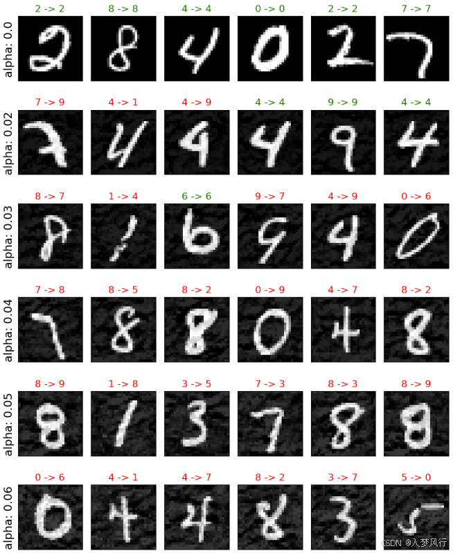
2.8 效果展示

def plot_adv_examples(adv_examples_list, epsilons):
    """展示对抗攻击效果"""
    cnt = 0
    plt.figure(figsize=(8, 10))
    for i in range(len(epsilons)):
        for j in range(len(adv_examples_list[i])):
            cnt += 1
            plt.subplot(len(epsilons), len(adv_examples_list[0]), cnt)
            plt.xticks([], [])
            plt.yticks([], [])
            if j == 0:
                plt.ylabel("alpha: {}".format(epsilons[i]/iterations), fontsize=14)
            orig_pred, adv_pred, adv_image = adv_examples_list[i][j]
            plt.title("{} -> {}".format(orig_pred, adv_pred),color=("green" if orig_pred==adv_pred else "red"))
            plt.imshow(adv_image, cmap="gray")
    plt.tight_layout()
    plt.show()

plot_adv_examples(adv_examples_list, epsilons)