TensorFlow进阶函数_import tensorflow as tf-优快云博客

本文链接：https://blog.youkuaiyun.com/qq_44004117/article/details/104858469

1、合并

1.1 拼接函数： tf.concat(tensors, axis)

tensors 保存了所有需要合并的张量 List；axis 指定需要合并的维度0、1、2（-1表示末尾）。注：对应合并的维度数值可以不同，其它维度必须相同。

import  os
os.environ['TF_CPP_MIN_LOG_LEVEL']='2'
import  tensorflow as tf
a = tf.random.normal([4,35,8]) # 模拟成绩册 A
b = tf.random.normal([6,35,8]) # 模拟成绩册 B
c = tf.concat([a,b],axis=0) # 合并成绩册
print(c)

1.2 堆叠：tf.stack(tensors, axis)函数。需要所有合并的张量 shape 完全一致才可堆叠。

import  os
os.environ['TF_CPP_MIN_LOG_LEVEL']='2'
import  tensorflow as tf
a = tf.random.normal([35,8])
b = tf.random.normal([35,8])
c = tf.stack([a,b],axis=0) # 堆叠合并为 2 个班级
d = tf.stack([a,b],axis=1) 
e = tf.stack([a,b],axis=2) 
print(c.shape,d.shape,e.shape)

1.3 分割：

分割函数tf.split(x, axis, num_or_size_splits)，x：待分割张量，axis：分割的维度索引号，num_or_size_splits：切割方案。

tf.unstack(x,axis)函数的作用：在某个维度上全部按长度为 1 的方式分割。

import  os
os.environ['TF_CPP_MIN_LOG_LEVEL']='2'
import  tensorflow as tf
x = tf.random.normal([10,6,7])
# 等长切割
b = tf.split(x,axis=0,num_or_size_splits=2)
d = tf.split(x,axis=0,num_or_size_splits=[4,2,2,2])
e = tf.unstack(x,axis=1)
c = len(e)
print(c,e[0].shape)

2、数据统计

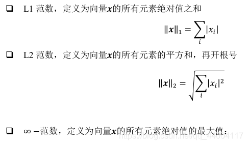
2.1 tf.norm(x,ord)函数：计算向量范数。

首先介绍一下范数的概念：

import  os
os.environ['TF_CPP_MIN_LOG_LEVEL']='2'
import  tensorflow as tf
import numpy as np
x = tf.ones([2,2])
a = tf.norm(x,ord=1) # 计算 L1 范数
b = tf.norm(x,ord=2) # 计算 L2 范数
c = tf.norm(x,ord=np.inf) # 计算∞范数
print(a,b,c)

2.2 tf.reduce_max, tf.reduce_min, tf.reduce_mean, tf.reduce_sum 可以求解张量在某个维度上的最大、最小、均值、和，也可以求全局最大、最小、均值、和信息。

当不指定 axis 参数时，tf.reduce_*函数会求解出全局元素的最大、最小、均值、和。

import  os
os.environ['TF_CPP_MIN_LOG_LEVEL']='2'
import  tensorflow as tf
import numpy as np
x = tf.random.normal([4,10])
a = tf.reduce_max(x,axis=1) # 统计概率维度上的最大值
b = tf.reduce_min(x,axis=1) # 统计概率维度上的最小值
c = tf.reduce_mean(x,axis=1) # 统计概率维度上的均值
d = tf.reduce_max(x)
print(a,b,c,d)

2.2.1 tf.reduce_mean()计算样本的平均误差：

import  os
os.environ['TF_CPP_MIN_LOG_LEVEL']='2'
import  tensorflow as tf
from tensorflow import keras
#from keras import losses
out = tf.random.normal([4,10]) # 网络预测输出
y = tf.constant([1,2,2,0]) # 真实标签
y = tf.one_hot(y,depth=10) # one-hot 编码
loss = keras.losses.mse(y,out) # 计算每个样本的误差
loss_f = tf.reduce_mean(loss) # 平均误差
print(y,loss,loss_f)

2.2.2 tf.reduce_sum(x,axis)函数求解张量在 axis 轴上所有特征的和：

import  os
os.environ['TF_CPP_MIN_LOG_LEVEL']='2'
import  tensorflow as tf
from tensorflow import keras
out = tf.random.normal([4,10])
a = tf.reduce_sum(out,axis=-1) # 求和
print(a)

2.2.3 tf.nn.softmax(out, axis=*)函数：获取最值所在的索引号。

import  os
os.environ['TF_CPP_MIN_LOG_LEVEL']='2'
import  tensorflow as tf
from tensorflow import keras
out = tf.random.normal([2,10])
out = tf.nn.softmax(out, axis=1) # 通过 softmax 转换为概率值
print(out,tf.reduce_sum(out[0]))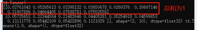

2.2.4 tf.argmax(x, axis)，tf.argmin(x, axis)可以求解在 axis 轴上，x 的最大值、最小值所在的索引号：

import  os
os.environ['TF_CPP_MIN_LOG_LEVEL']='2'
import  tensorflow as tf
out = tf.random.normal([2,10])
pred = tf.argmax(out, axis=1) # 选取概率最大的位置
print(pred)

输出结果如下：

3、张量比较

tf.equal(a, b)(或 tf.math.equal(a, b))函数可以比较 2个张量是否相等。

import  os
os.environ['TF_CPP_MIN_LOG_LEVEL']='2'
import  tensorflow as tf
out = tf.random.normal([100,10])
out = tf.nn.softmax(out, axis=1) # 输出转换为概率
pred = tf.argmax(out, axis=1) # 选取预测值
y = tf.random.uniform([100],dtype=tf.int64,maxval=10)
out = tf.equal(pred,y) # 预测值与真实值比较
out1 = tf.cast(out, dtype=tf.int32) # 布尔型转 int 型
correct = tf.reduce_sum(out1) # 统计 True 的个数
print(pred,y,out,out1,correct)

4、填充和复制

tf.pad(x, paddings)函数：填充

paddings 是包含了多个[left padding,right padding]的嵌套方案 List。

import  os
os.environ['TF_CPP_MIN_LOG_LEVEL']='2'
import  tensorflow as tf
a = tf.constant([1,2,3,4,5,6,7,8])
b = tf.constant([7,8,1,6])
b = tf.pad(b, [[1,3]]) # 填充
print(b)

tf.tile 函数可以在任意维度将数据重复复制多份。

import  os
os.environ['TF_CPP_MIN_LOG_LEVEL']='2'
import  tensorflow as tf
x = tf.random.normal([4,32,32,3])
b = tf.tile(x,[2,3,3,1]) # 数据复制
print(b.shape)

结果如下：

5、数据限幅

tf.maximum(x, a)实现数据的下限幅：𝑦 ∈ [𝑏,+∞)

tf.minimum(x, a)实现数据的上限幅：𝑦 ∈ (−∞,𝑏]

组合 tf.maximum(x, a)和 tf.minimum(x, b)可以实现同时对数据的上下边界限幅：𝑦 ∈ [a,b]

import  os
os.environ['TF_CPP_MIN_LOG_LEVEL']='2'
import  tensorflow as tf
x = tf.range(9)
a = tf.maximum(x,2) # 下限幅2
b = tf.minimum(x,7) # 上限幅 7
c = tf.minimum(tf.maximum(x,2),7) # 限幅为 2~7
print(a,b,c)

6、高级操作

tf.gather 可以实现根据索引号收集数据的目的。

import  os
os.environ['TF_CPP_MIN_LOG_LEVEL']='2'
import  tensorflow as tf
x = tf.random.uniform([4,35,8],maxval=100,dtype=tf.int32)
a = tf.gather(x,[0,1],axis=0) # 在班级维度收集第 1-2 号班级成绩册
print(a)

tf.gather_nd，可以通过指定每次采样的坐标来实现采样多个点的目的。

import  os
os.environ['TF_CPP_MIN_LOG_LEVEL']='2'
import  tensorflow as tf
x = tf.random.uniform([4,35,8],maxval=100,dtype=tf.int32)
# 根据多维度坐标收集数据
a = tf.gather_nd(x,[[1,1],[2,2],[3,3]])			# 班级 1，学生 1 的所有科目
b = tf.gather_nd(x,[[1,1,2],[2,2,3],[3,3,4]]) 	# 班级 1，学生 1 的科目 2
print(a)

tf.boolean_mask(x, mask, axis)可以在 axis 轴上根据 mask 方案进行采样。

import  os
os.environ['TF_CPP_MIN_LOG_LEVEL']='2'
import  tensorflow as tf
x = tf.random.uniform([4,35,8],maxval=100,dtype=tf.int32)
# 根据掩码方式采样班级
a = tf.boolean_mask(x,mask=[True, False,False,True],axis=0)
# 根据掩码方式采样科目
b = tf.boolean_mask(x,mask=[True,False,False,True,True,False,False,True],axis=2)
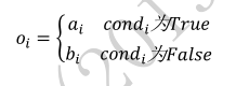
print(a.shape,b.shape)

tf.where(cond, a, b)操作可以根据 cond 条件的真假从 a 或 b 中读取数据，条件判定规则如下：

import  os
os.environ['TF_CPP_MIN_LOG_LEVEL']='2'
import  tensorflow as tf
a = tf.ones([3,3]) # 构造 a 为全 1
b = tf.zeros([3,3]) # 构造 b 为全 0
cond = tf.constant([[True,False,False],[False,True,False],[True,True,False]])
c = tf.where(cond,a,b) # 根据条件从 a,b 中采样
print(c)

提取张量中所有正数的数据和索引：

import  os
os.environ['TF_CPP_MIN_LOG_LEVEL']='2'
import  tensorflow as tf
x = tf.random.normal([3,3]) # 构造a
mask=x>0 # 比较操作，等同于 tf.equal()
indices=tf.where(mask) # 提取所有大于 0 的元素索引
a = tf.gather_nd(x,indices) # 提取正数的元素值
b = tf.boolean_mask(x,mask) # 通过掩码提取正数的元素值
print(x,mask,indices,a,b)	# a = b

tf.scatter_nd(indices, updates, shape)可以高效地刷新张量的部分数据

import  os
os.environ['TF_CPP_MIN_LOG_LEVEL']='2'
import  tensorflow as tf
# 构造需要刷新数据的位置
indices = tf.constant([[4], [3], [1], [7]])
# 构造需要写入的数据
updates = tf.constant([4.4, 3.3, 1.1, 7.7])
# 在长度为 8 的全 0 向量上根据 indices 写入 updates
a = tf.scatter_nd(indices, updates, [8])
print(a)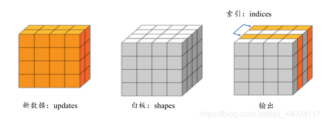

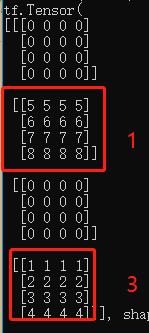
import  os
os.environ['TF_CPP_MIN_LOG_LEVEL']='2'
import  tensorflow as tf
# 构造写入位置
indices = tf.constant([[1],[3]])
updates = tf.constant([							# 构造写入数据
[[5,5,5,5],[6,6,6,6],[7,7,7,7],[8,8,8,8]],
[[1,1,1,1],[2,2,2,2],[3,3,3,3],[4,4,4,4]]
])
# 在 shape 为[4,4,4]白板上根据 indices 写入 updates
a = tf.scatter_nd(indices,updates,[4,4,4])
print(a)

结果如下：

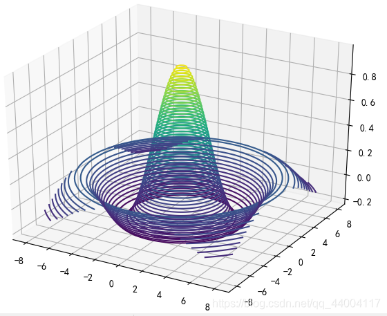
tf.meshgrid()函数生成二维网格采样点坐标，并通过Axes3d绘制三维图。

import  os
os.environ['TF_CPP_MIN_LOG_LEVEL']='2'
import  tensorflow as tf
import matplotlib.pyplot as plt
from mpl_toolkits.mplot3d import Axes3D
x = tf.linspace(-8.,8,100) # 设置 x 坐标的间隔
y = tf.linspace(-8.,8,100) # 设置 y 坐标的间隔
x,y = tf.meshgrid(x,y) # 生成网格点，并拆分后返回
z = tf.sqrt(x**2+y**2)
z = tf.sin(z)/z # sinc 函数实现
print(x.shape,y.shape)		# 打印拆分后的所有点的 x,y 坐标张量 shape
fig = plt.figure()
ax = Axes3D(fig)
# 根据网格点绘制 sinc 函数 3D 曲面
ax.contour3D(x.numpy(), y.numpy(), z.numpy(), 50)
plt.show()

结果如下：

7、经典数据集加载

keras.datasets 模块提供了常用经典数据集的自动下载、管理、加载与转换功能，并且提供了 tf.data.Dataset 数据集对象。

datasets.xxx.load_data()即可实现经典数据集的自动加载，其中 xxx 代表具体的数据集名称。

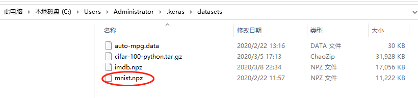
TensorFlow 会默认将数据缓存在用户目录下的.keras/datasets 文件夹。

如果当前数据集不在缓存中，则会自动从网站下载和解压，加载；如果已经在缓存中，自动完成加载：

import  os
os.environ['TF_CPP_MIN_LOG_LEVEL']='2'
import tensorflow as tf
from tensorflow import keras
from tensorflow.keras import datasets # 导入经典数据集加载模块
# 加载 MNIST 数据集
(x, y), (x_test, y_test) = datasets.mnist.load_data()
print('x:', x.shape, 'y:', y.shape, 'x test:', x_test.shape, 'y test:',y_test)

通过 load_data()会返回相应格式的数据，对于图片数据集 MNIST, CIFAR10 等，会返回 2个 tuple，第一个 tuple 保存了用于训练的数据 x,y 训练集对象；第 2 个 tuple 则保存了用于测试的数据 x_test,y_test 测试集对象，所有的数据都用 Numpy.array 容器承载。

随机打散、批训练、预处理：

import  os
os.environ['TF_CPP_MIN_LOG_LEVEL']='2'
import tensorflow as tf
from tensorflow import keras
from tensorflow.keras import datasets # 导入经典数据集加载模块
# 加载 MNIST 数据集
(x, y), (x_test, y_test) = datasets.mnist.load_data()
# 转换成 Dataset 对象
train_db = tf.data.Dataset.from_tensor_slices((x, y))
# 随机打散
train_db = train_db.shuffle(10000)
train_db = train_db.batch(128)		#  128 为 batch size 参数，即一次并行计算 128 个样本的数据。
def preprocess(x, y): # 自定义的预处理函数
	# 调用此函数时会自动传入 x,y 对象，shape 为[b, 28, 28], [b]
	# 标准化到 0~1
	x = tf.cast(x, dtype=tf.float32) / 255.
	x = tf.reshape(x, [-1, 28*28]) # 打平
	y = tf.cast(y, dtype=tf.int32) # 转成整形张量
	y = tf.one_hot(y, depth=10) # one-hot 编码
	# 返回的 x,y 将替换传入的 x,y 参数，从而实现数据的预处理功能
	return x,y
# 预处理函数实现在 preprocess 函数中，传入函数引用即可
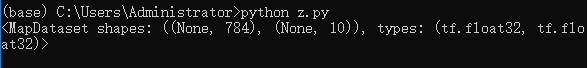
train_db = train_db.map(preprocess)
print(train_db)

3个输出结果如下：

8、循环训练

# 方法一
for epoch in range(20): # 训练 Epoch 数
for step, (x,y) in enumerate(train_db): # 迭代 Step 数
# training...
# 方法二：
train_db = train_db.repeat(20) # 数据集迭代 20 遍才终止

9、MNIST 测试实战

#%%
import  matplotlib
from    matplotlib import pyplot as plt
# Default parameters for plots
matplotlib.rcParams['font.size'] = 20
matplotlib.rcParams['figure.titlesize'] = 20
matplotlib.rcParams['figure.figsize'] = [9, 7]
# matplotlib.rcParams['font.family'] = ['STKaiTi']
matplotlib.rcParams['axes.unicode_minus']=False 
import  tensorflow as tf
from    tensorflow import keras
from    tensorflow.keras import datasets, layers, optimizers
import  os

os.environ['TF_CPP_MIN_LOG_LEVEL']='2'
print(tf.__version__)

def preprocess(x, y): 
    # [b, 28, 28], [b]
    print(x.shape,y.shape)
    x = tf.cast(x, dtype=tf.float32) / 255.
    x = tf.reshape(x, [-1, 28*28])
    y = tf.cast(y, dtype=tf.int32)
    y = tf.one_hot(y, depth=10)

    return x,y

#%%
(x, y), (x_test, y_test) = datasets.mnist.load_data()
print('x:', x.shape, 'y:', y.shape, 'x test:', x_test.shape, 'y test:', y_test)
#%%
batchsz = 512
train_db = tf.data.Dataset.from_tensor_slices((x, y))
train_db = train_db.shuffle(1000)
train_db = train_db.batch(batchsz)
train_db = train_db.map(preprocess)
train_db = train_db.repeat(20)

#%%

test_db = tf.data.Dataset.from_tensor_slices((x_test, y_test))
test_db = test_db.shuffle(1000).batch(batchsz).map(preprocess)
x,y = next(iter(train_db))
print('train sample:', x.shape, y.shape)
# print(x[0], y[0])

#%%
def main():

    # learning rate
    lr = 1e-2
    accs,losses = [], []


    # 784 => 512
    w1, b1 = tf.Variable(tf.random.normal([784, 256], stddev=0.1)), tf.Variable(tf.zeros([256]))
    # 512 => 256
    w2, b2 = tf.Variable(tf.random.normal([256, 128], stddev=0.1)), tf.Variable(tf.zeros([128]))
    # 256 => 10
    w3, b3 = tf.Variable(tf.random.normal([128, 10], stddev=0.1)), tf.Variable(tf.zeros([10])) 

    for step, (x,y) in enumerate(train_db):
 
        # [b, 28, 28] => [b, 784]
        x = tf.reshape(x, (-1, 784))

        with tf.GradientTape() as tape:

            # layer1.
            h1 = x @ w1 + b1
            h1 = tf.nn.relu(h1)
            # layer2
            h2 = h1 @ w2 + b2
            h2 = tf.nn.relu(h2)
            # output
            out = h2 @ w3 + b3
            # out = tf.nn.relu(out)

            # compute loss
            # [b, 10] - [b, 10]
            loss = tf.square(y-out)
            # [b, 10] => scalar
            loss = tf.reduce_mean(loss)

 
        grads = tape.gradient(loss, [w1, b1, w2, b2, w3, b3]) 
        for p, g in zip([w1, b1, w2, b2, w3, b3], grads):
            p.assign_sub(lr * g)


        # print
        if step % 80 == 0:
            print(step, 'loss:', float(loss))
            losses.append(float(loss))
 
        if step %80 == 0:
            # evaluate/test
            total, total_correct = 0., 0

            for x, y in test_db:
                # layer1.
                h1 = x @ w1 + b1
                h1 = tf.nn.relu(h1)
                # layer2
                h2 = h1 @ w2 + b2
                h2 = tf.nn.relu(h2)
                # output
                out = h2 @ w3 + b3
                # [b, 10] => [b]
                pred = tf.argmax(out, axis=1)
                # convert one_hot y to number y
                y = tf.argmax(y, axis=1)
                # bool type
                correct = tf.equal(pred, y)
                # bool tensor => int tensor => numpy
                total_correct += tf.reduce_sum(tf.cast(correct, dtype=tf.int32)).numpy()
                total += x.shape[0]

            print(step, 'Evaluate Acc:', total_correct/total)

            accs.append(total_correct/total)

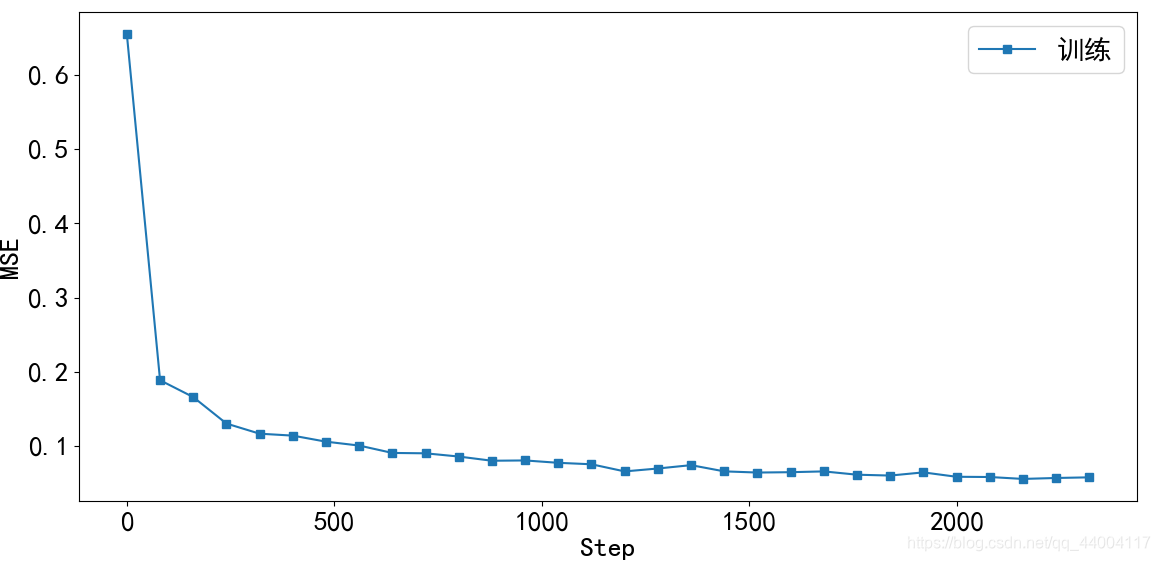
    plt.figure()
    x = [i*80 for i in range(len(losses))]
    plt.plot(x, losses, color='C0', marker='s', label='训练')
    plt.ylabel('MSE')
    plt.xlabel('Step')
    plt.legend()
    plt.savefig('train.svg')
    plt.show()

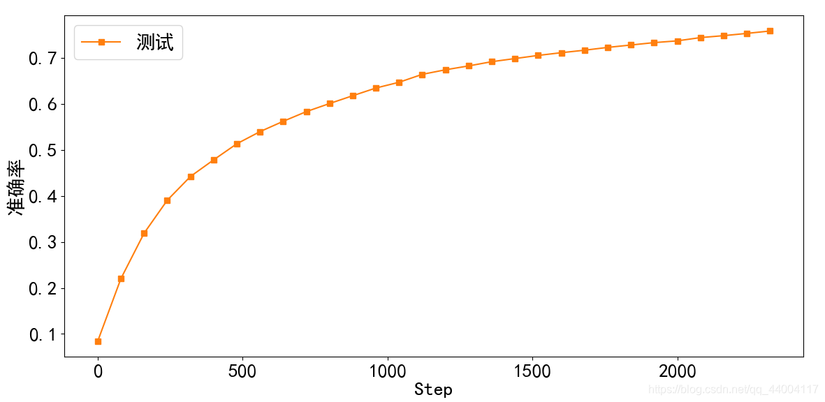
    plt.figure()
    plt.plot(x, accs, color='C1', marker='s', label='测试')
    plt.ylabel('准确率')
    plt.xlabel('Step')
    plt.legend()
    plt.savefig('test.svg')
    plt.show()

if __name__ == '__main__':
    main()

输出1：

输出2：