pytorh入门

一、pytorch基础知识

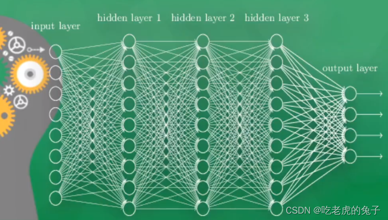
1.1 神经网络简介

模拟生物学的人脑的神经元进行组装
神经网络可以大致分为输入层-隐藏层-输出层

1.2 梯度下降

梯度下降，可以理解为下降到梯度线“躺平”的点
一般情况下神经网络中会有很多个W进行梯度下降，

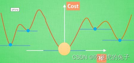
但是问题可能在，当找到“躺平”点的时候会出现在一个局部最优解，而找不到全局最优解，当然这是无法避免的，但是只要局部足够优秀的情况下也可以得到很好的效果。

1.3 numpy和pytorch

让我们来看一下numpy和torch打印出来的区别，以及tensor和numpy之间的转换

import torch
import numpy as np
np_data = np.arange(6).reshape((2,3))
torch_data = torch.from_numpy(np_data)
tensorToArray = torch_data.numpy()
print(
    '\nnumpy',np_data,
    '\ntorch',torch_data,
    '\ntensorToArray',tensorToArray,
)

numpy [[0 1 2]
 [3 4 5]] 
torch tensor([[0, 1, 2],
        [3, 4, 5]], dtype=torch.int32) 
tensorToArray [[0 1 2]
 [3 4 5]]

一些numpy和torch的功能对比（abs、sin、mean）

import torch
import numpy as np
# abs
data = [-1,-2,1,2]
tensor = torch.FloatTensor(data)
print(
    '\nabs',
    '\nnumpy',np.abs(data),
    '\ntorch',torch.abs(tensor)
)
# sin
print(
    '\nsin',
    '\nnumpy',np.sin(data),
    '\ntorch',torch.sin(tensor)
)
# mean
print(
    '\nmean',
    '\nnumpy',np.mean(data),
    '\ntorch',torch.mean(tensor)
)

abs 
numpy [1 2 1 2] 
torch tensor([1., 2., 1., 2.])

sin 
numpy [-0.84147098 -0.90929743  0.84147098  0.90929743] 
torch tensor([-0.8415, -0.9093,  0.8415,  0.9093])

mean 
numpy 0.0 
torch tensor(0.)

1.4 pytorch中的变量——Variable

可以把Variable想象成一个盒子，里边装了很多个tensor变量，通过对变量的计算，那么variable可以同时计算他的梯度等信息。
以下是variable的一些属性

import torch
import numpy as np
from torch.autograd import Variable
tensor = torch.FloatTensor([[1,2],[3,4]])
variable = Variable(tensor,requires_grad=True)
print(variable)
print(tensor)
t_out = torch.mean(tensor*tensor)
v_out = torch.mean(variable*variable)
print(t_out)
print(v_out)
v_out.backward()
print(variable.grad)
print(variable.data)
print(variable.data.numpy())

tensor([[1., 2.],
        [3., 4.]], requires_grad=True)
tensor([[1., 2.],
        [3., 4.]])
tensor(7.5000)
tensor(7.5000, grad_fn=<MeanBackward0>)
tensor([[0.5000, 1.0000],
        [1.5000, 2.0000]])
tensor([[1., 2.],
        [3., 4.]])
[[1. 2.]
 [3. 4.]]

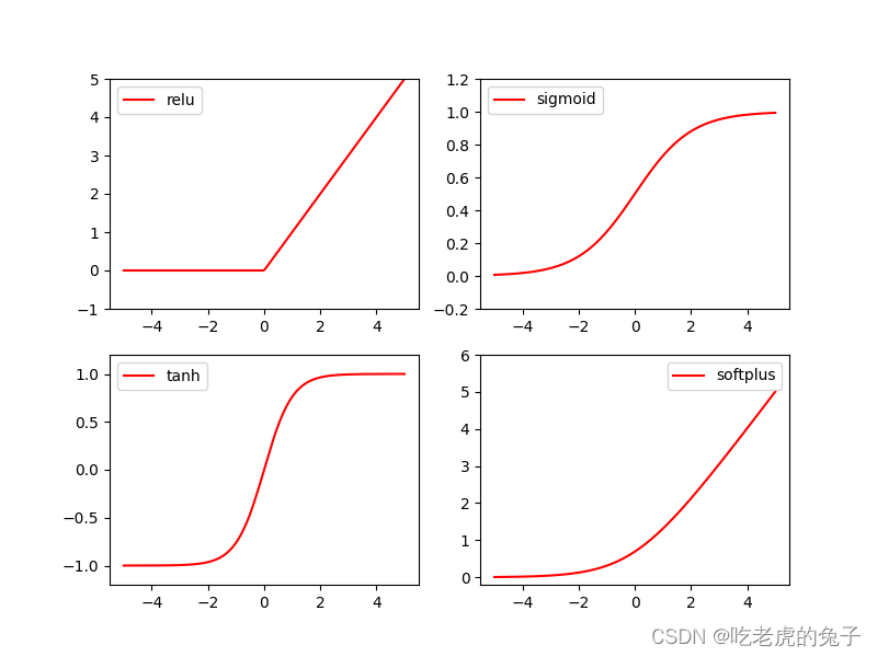
1.5 激励函数

• relu
  y_relu = F.relu(x).data.numpy()
• sigmoid
  y_sigmoid = F.sigmoid(x).data.numpy()
• tanh
  y_tanh = F.tanh(x).data.numpy()
• softmax
  y_softplus = F.softplus(x).data.numpy()
  

二、建立一个初级神经网络

2.1 关系拟合

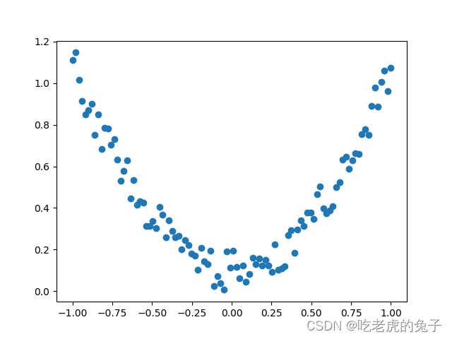
2.1.1 随机生成一些数据集中的数据

x = torch.unsqueeze(torch.linspace(-1,1,100),dim=1)
y = x.pow(2) + 0.2*torch.rand(x.size())

x,y = Variable(x), Variable(y)

plt.scatter(x.data.numpy(),y.data.numpy())
plt.show()

2.1.2 建立神经网络

class Net(torch.nn.Module):
    def __init__(self,n_feature,n_hidden,n_output):
        super(Net,self).__init__()
        self.hidden = torch.nn.Linear(n_feature,n_hidden)
        self.predict = torch.nn.Linear(n_hidden, n_output)
    def forward(self,x):
        x = F.relu(self.hidden(x))
        x = self.predict(x)
        return x
net = Net(n_feature=1, n_hidden=10, n_output=1)
print(net)

Net(
  (hidden): Linear(in_features=1, out_features=10, bias=True)
  (predict): Linear(in_features=10, out_features=1, bias=True)
)

2.1.3 可视化训练过程

#!/usr/bin/python
# -*- coding:utf8 -*-

import torch
from torch.autograd import Variable
import torch.nn.functional as F
import matplotlib.pyplot as plt

x = torch.unsqueeze(torch.linspace(-1,1,100),dim=1)
y = x.pow(2) + 0.2*torch.rand(x.size())

x,y = Variable(x), Variable(y)

# plt.scatter(x.data.numpy(),y.data.numpy())
# plt.show()

class Net(torch.nn.Module):
    def __init__(self,n_feature,n_hidden,n_output):
        super(Net,self).__init__()
        self.hidden = torch.nn.Linear(n_feature,n_hidden)
        self.predict = torch.nn.Linear(n_hidden, n_output)

    def forward(self,x):
        x = F.relu(self.hidden(x))
        x = self.predict(x)
        return x

net = Net(n_feature=1, n_hidden=10, n_output=1)
print(net)

# 学习器
optimizer = torch.optim.SGD(net.parameters(),lr=0.5)
loss_func = torch.nn.MSELoss() # 均方差

plt.ion()
plt.show()

for t in range(100):
    prediction = net(x) # 预测结果
    loss = loss_func(prediction,y) # 计算损失
    optimizer.zero_grad() # 将梯度降为0
    loss.backward() # 反向传递
    optimizer.step() # 优化梯度
    if t % 5 == 0:
        plt.cla()
        plt.scatter(x.data.numpy(),y.data.numpy())
        plt.plot(x.data.numpy(),prediction.data.numpy())
        plt.text(0.5,0,'Loss=%.4f'%loss.data.numpy(),fontdict={'size': 20, 'color':  'red'})
        plt.pause(0.1)

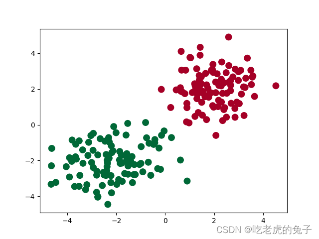
2.2 区分类型

2.2.1 生成数据集

import torch
import matplotlib.pyplot as plt
# 假数据
n_data = torch.ones(100, 2)         # 数据的基本形态
x0 = torch.normal(2*n_data, 1)      # 类型0 x data (tensor), shape=(100, 2)
y0 = torch.zeros(100)               # 类型0 y data (tensor), shape=(100, )
x1 = torch.normal(-2*n_data, 1)     # 类型1 x data (tensor), shape=(100, 1)
y1 = torch.ones(100)                # 类型1 y data (tensor), shape=(100, )
# 注意 x, y 数据的数据形式是一定要像下面一样 (torch.cat 是在合并数据)
x = torch.cat((x0, x1), 0).type(torch.FloatTensor)  # FloatTensor = 32-bit floating
y = torch.cat((y0, y1), ).type(torch.LongTensor)    # LongTensor = 64-bit integer
plt.scatter(x.data.numpy()[:, 0], x.data.numpy()[:, 1], c=y.data.numpy(), s=100, lw=0, cmap='RdYlGn')
plt.show()

2.2.2 建立神经网络

class Net(torch.nn.Module):
    def __init__(self,n_feature,n_hidden,n_output):
        super(Net,self).__init__()
        self.hidden = torch.nn.Linear(n_feature,n_hidden)
        self.out = torch.nn.Linear(n_hidden,n_output)

    def forward(self,x):
        x = F.relu(self.hidden(x))
        x = self.out(x)
        return x

net = Net(n_feature=2,n_hidden=10,n_output=2)
print(net)

Net(
  (hidden): Linear(in_features=2, out_features=10, bias=True)
  (out): Linear(in_features=10, out_features=2, bias=True)
)

2.2.3 可视化训练网络

#!/usr/bin/python
# -*- coding:utf8 -*-

import torch
import matplotlib.pyplot as plt
import torch.nn.functional as F

# 假数据
n_data = torch.ones(100, 2)         # 数据的基本形态
x0 = torch.normal(2*n_data, 1)      # 类型0 x data (tensor), shape=(100, 2)
y0 = torch.zeros(100)               # 类型0 y data (tensor), shape=(100, )
x1 = torch.normal(-2*n_data, 1)     # 类型1 x data (tensor), shape=(100, 1)
y1 = torch.ones(100)                # 类型1 y data (tensor), shape=(100, )

# 注意 x, y 数据的数据形式是一定要像下面一样 (torch.cat 是在合并数据)
x = torch.cat((x0, x1), 0).type(torch.FloatTensor)  # FloatTensor = 32-bit floating
y = torch.cat((y0, y1), ).type(torch.LongTensor)    # LongTensor = 64-bit integer

plt.scatter(x.data.numpy()[:, 0], x.data.numpy()[:, 1], c=y.data.numpy(), s=100, lw=0, cmap='RdYlGn')
plt.show()

# 建立神经网络
class Net(torch.nn.Module):
    def __init__(self,n_feature,n_hidden,n_output):
        super(Net,self).__init__()
        self.hidden = torch.nn.Linear(n_feature,n_hidden)
        self.out = torch.nn.Linear(n_hidden,n_output)

    def forward(self,x):
        x = F.relu(self.hidden(x))
        x = self.out(x)
        return x

net = Net(n_feature=2,n_hidden=10,n_output=2)
print(net)

optimier = torch.optim.SGD(net.parameters(),lr = 0.02)
loss_func = torch.nn.CrossEntropyLoss()

for t in range(100):
    out = net(x)
    loss = loss_func(out,y)
    optimier.zero_grad()
    loss.backward()
    optimier.step()
    if t%2 == 0:
        plt.cla()
        prediction = torch.max(F.softmax(out), 1)[1]
        pre_y = prediction.data.numpy().squeeze()
        target_y = y.data.numpy()
        plt.scatter(x.data.numpy()[:,0],x.data.numpy()[:,1],c=pre_y,s=100,lw=0,cmap='RdYlGn')
        accuracy = sum(pre_y == target_y)/200.
        plt.text(1.5, -4, 'Accuracy=%.2f' % accuracy, fontdict={'size': 20, 'color': 'red'})
        plt.pause(0.1)

2.3 模型的保存和使用

# 保存网络
torch.save(net1, 'net.pkl')  # 保存整个网络
torch.save(net1.state_dict(), 'net_params.pkl')   # 只保存网络中的参数 (速度快, 占内存少)

# 使用方法1
def restore_net():
    # restore entire net1 to net2
    net2 = torch.load('net.pkl')
    prediction = net2(x)
# 使用方式2
def restore_params():
    # 新建 net3
    net3 = torch.nn.Sequential(
        torch.nn.Linear(1, 10),
        torch.nn.ReLU(),
        torch.nn.Linear(10, 1)
    )
    # 将保存的参数复制到 net3
    net3.load_state_dict(torch.load('net_params.pkl'))
    prediction = net3(x)

2.4 批训练

DataLoader
它可以包装自己的数据, 进行批训练

#!/usr/bin/python
# -*- coding:utf8 -*-
import torch
import torch.utils.data as Data
def train():
    BATCH_SIZE = 5
    # linspace 线性间距向量 - tensor类型
    # start,emd,step
    # 从start开始到end结束 一共平均分成step份
    x = torch.linspace(1, 10, 10)
    y = torch.linspace(10, 1, 10)
    # 将tensor转换成dataset
    torch_dataset = Data.TensorDataset(x, y)
    # 使用DataLoader装饰器
    loader = Data.DataLoader(
        dataset=torch_dataset,# 数据集
        batch_size=BATCH_SIZE, #每次读取多少个数据
        shuffle=True, # 是否打乱读取
        num_workers=2, # 多线程读取
    )
    for epoch in range(3):  # 打乱整套数据三次
        for step, (batch_x, batch_y) in enumerate(loader):
            # training......
            print('Epoch:', epoch, '|Step:', step, '|batch x:',
                  batch_x.numpy(), '|batch y:', batch_y.numpy)
if __name__ == '__main__':
    train()

tensor([ 1.,  2.,  3.,  4.,  5.,  6.,  7.,  8.,  9., 10.])
tensor([10.,  9.,  8.,  7.,  6.,  5.,  4.,  3.,  2.,  1.])
Epoch: 0 |Step: 0 |batch x: [2. 6. 7. 9. 3.] |batch y: <built-in method numpy of Tensor object at 0x000002E0465AE9A8>
Epoch: 0 |Step: 1 |batch x: [ 1. 10.  8.  5.  4.] |batch y: <built-in method numpy of Tensor object at 0x000002E0465AEF48>
Epoch: 1 |Step: 0 |batch x: [8. 4. 2. 5. 7.] |batch y: <built-in method numpy of Tensor object at 0x000002E0466D92C8>
Epoch: 1 |Step: 1 |batch x: [ 3.  6.  1.  9. 10.] |batch y: <built-in method numpy of Tensor object at 0x000002E0466D9278>
Epoch: 2 |Step: 0 |batch x: [8. 7. 4. 6. 9.] |batch y: <built-in method numpy of Tensor object at 0x000002E0466D9368>
Epoch: 2 |Step: 1 |batch x: [ 2.  1.  5.  3. 10.] |batch y: <built-in method numpy of Tensor object at 0x000002E0466D9228>

2.5 加速神经网络

2.5.1 SGD ( Stochastic Gradient Descent )

将data分成许多块小的部分后再扔进网络结构中，这样虽然不能反映整体数据情况，但是却可以加速NN训练过程，并且也不会丢失太多准确率

2.5.2 momentum

（更改学习率）
传统的参数 W 的更新是把原始的 W 累加上一个负的学习率(learning rate) 乘以校正值 (dx)。这种方法可能会让学习过程曲折无比, 看起来像 喝醉的人回家时, 摇摇晃晃走了很多弯路。
w+=-learning rate * dx

所以我们把这个人从平地上放到了一个斜坡上, 只要他往下坡的方向走一点点, 由于向下的惯性, 他不自觉地就一直往下走, 走的弯路也变少了。
m=b1*m-learning rate * dx
w+=m

2.5.3 AdaGrad

给权值一个阻力，让他只能往前走而不是横向的走，这样能够更快的进行梯度下降。

2.5.4 RMSProp

结合上述的AdaGrad和momentum方法

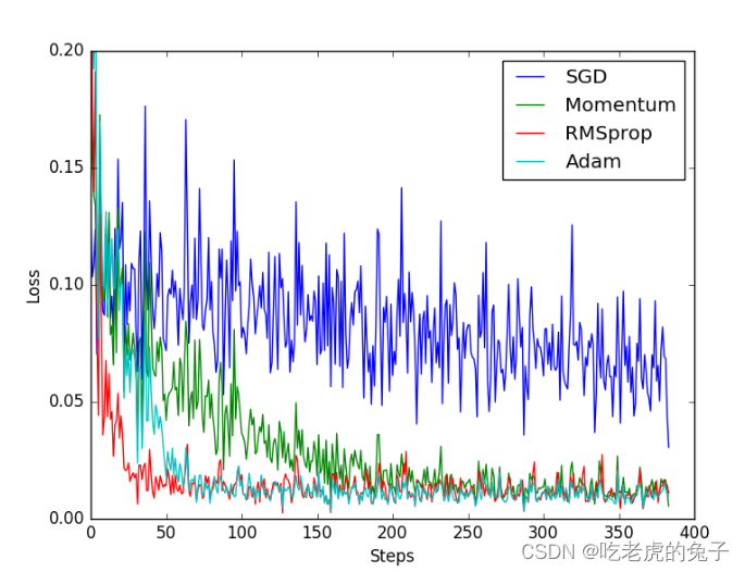
2.6 Optimizer优化器

opt_SGD         = torch.optim.SGD(net_SGD.parameters(), lr=LR)
opt_Momentum    = torch.optim.SGD(net_Momentum.parameters(), lr=LR, momentum=0.8)
opt_RMSprop     = torch.optim.RMSprop(net_RMSprop.parameters(), lr=LR, alpha=0.9)
opt_Adam        = torch.optim.Adam(net_Adam.parameters(), lr=LR, betas=(0.9, 0.99))

三、高级神经网络

3.1 卷积神经网络CNN介绍

一个常见的对于图片处理的卷积神经网络结构：
图片输入-卷积层-池化层-卷积层-池化层-全连接层-全连接层-分类器输出
以图片处理的过程为例
卷积-每次神经元都提取完整图片中的一小部分学习特征，这个就是卷积的过程。
池化-由于卷积的过程中会无意的丢掉一些数据，这时候就需要池化层来帮助解决了，池化是一个筛选过滤的过程, 能将 layer 中有用的信息筛选出来, 给下一个层分析。

3.2 卷积神经网络CNN实现

import torchvision
import matplotlib.pyplot as plt
import random
# 设置超参数
EPOCH = 3  # 训练的轮数
BATCH_SIZE = 50  # 每个批次的数据量
LR = 0.001  # 学习率
DOWNLOAD_MINIST = True # 是否下在 如果已经下载了 就把这里改成False
if __name__ == '__main__':
	# 数据集
    train_data = torchvision.datasets.MNIST(
        root='./minist',
        train=True,
        transform=torchvision.transforms.ToTensor(),  # 将（0，255）压缩到（0，1）
        download=DOWNLOAD_MINIST,
    )
    x = random.randint(0,10000)
    # 呈现一下训练集的内容
    print(train_data.train_data.size())
    print(train_data.train_labels.size())
    plt.imshow(train_data.train_data[x], cmap='gray')
    plt.title("%i" % train_data.train_labels[x])
    plt.show()
# 建立CNN网络
    class CNN(nn.Module):
        def __init__(self):
            super(CNN,self).__init__()
            self.conv1 = nn.Sequential(
                nn.Conv2d(    # 1*28*28
                    # rgb的层次（这里MINIST数据集黑白颜色的，高度只有一层）
                    in_channels=1,
                    # 可以理解为有16个扫描器在扫描，每个扫描器都会提取出来一个信息，这样就会输出16个信息。
                    out_channels=16,
                    # 可以理解为这个扫描器大小为5*5
                    kernel_size=5,
                    # 步长
                    stride=1,
                    # 给原始图片周围围上两圈0
                    padding=2
                ), # 过滤器 每次通过移动来收集图片的各处的信息 # 16*28*28
                nn.ReLU(), # 一个激励函数 # 16*28*28
                # 一个过滤器，2*2的核，选择其中最大的值。之后将这个元素的图片变成更窄的图 但是高度不变。
                nn.MaxPool2d(kernel_size=2)  # 16*14*14
            )
            self.conv2 = nn.Sequential(
                nn.Conv2d(16,32,5,1,2), # 32*14*14
                nn.ReLU(), # 32*14*14
                nn.MaxPool2d(2) # 32*7*7
            )
            self.out = nn.Linear(32 * 7 * 7, 10)
        def forward(self,x):
            x = self.conv1(x)
            x = self.conv2(x)      # (batch 32,7,7)
            x = x.view(x.size(0),-1)     # (batch 32*7*7)
            output = self.out(x)
            return output
    cnn = CNN()
    print(cnn)
cnn = CNN()
    # print(cnn)
    optimizer = torch.optim.Adam(cnn.parameters(),lr=LR)
    loss_func = nn.CrossEntropyLoss()

    for epoch in range(EPOCH):
        for step,(b_x,b_y) in enumerate(train_loader):
            output = cnn(b_x)
            loss = loss_func(output,b_y)
            optimizer.zero_grad()
            loss.backward()
            optimizer.step()
            if step%500 == 0:
                test_output = cnn(test_x)
                pre_y = torch.max(test_output,1)[1].data.squeeze()
                accuracy = sum(pre_y == test_y) / test_y.size(0)
                print('Epoch:', epoch, '|train loss:',loss)
    test_output = cnn(test_x[:100])
    pre_y = torch.max(test_output,1)[1].data.numpy().squeeze()
    print(pre_y,'prediction number')
    print(test_y[:100].numpy(),'real number')

3.3 循环神经网络RNN的介绍

普通的网络NN只能对单个数据进行学习和处理，譬如data0对应的result0、data1对应的result1…
每一个result都是基于他的data来进行预测的
然而，当各个data相互之间存在相互关联之间的关系的时候，普通的NN就不再适用了。
这时候RNN就有用武之地了，RNN就会把之前的记忆都累积起来, 一起分析。

3.4 LSTM（LongShort-Term Memory）循环神经网络（分类）

使用mnist数据集

class RNN(nn.Module):
    def __init__(self):
        super(RNN, self).__init__()

        self.rnn = nn.LSTM(         # if use nn.RNN(), it hardly learns
            input_size=INPUT_SIZE,
            hidden_size=64,         # rnn hidden unit
            num_layers=1,           # number of rnn layer
            batch_first=True,       # input & output will has batch size as 1s dimension. e.g. (batch, time_step, input_size)
        self.out = nn.Linear(64, 10)
    def forward(self, x):
        # x shape (batch, time_step, input_size)
        # r_out shape (batch, time_step, output_size)
        # h_n shape (n_layers, batch, hidden_size)
        # h_c shape (n_layers, batch, hidden_size)
        r_out, (h_n, h_c) = self.rnn(x, None)   # None represents zero initial hidden state
        # choose r_out at the last time step
        out = self.out(r_out[:, -1, :])
        return out
rnn = RNN()
print(rnn)

RNN(
  (rnn): LSTM(28, 64, batch_first=True)
  (out): Linear(in_features=64, out_features=10, bias=True)
)

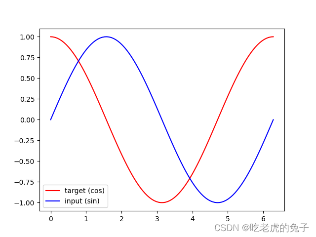
3.4 RNN循环神经网络（回归）

构建数据集（sin函数x cos函数y）

# show data
steps = np.linspace(0, np.pi*2, 100, dtype=np.float32)
x_np = np.sin(steps)
y_np = np.cos(steps)
plt.plot(steps, y_np, 'r-', label='target (cos)')
plt.plot(steps, x_np, 'b-', label='input (sin)')
plt.legend(loc='best')
plt.show()

构建网络

class RNN(nn.Module):
    def __init__(self):
        super(RNN, self).__init__()

        self.rnn = nn.RNN(
            input_size=INPUT_SIZE, # 输入一个时间点
            hidden_size=32,  # 隐藏层神经元个数
            num_layers=1,  # 数值越大计算能力越强 但是对计算机的消耗也越大
            batch_first=True,  # batch的维度是不是在第一个
        )
        self.out = nn.Linear(32, 1) # 因为是回归 所以输出到一个结果上

    def forward(self, x, h_state):
        # x (batch, time_step, input_size)
        # h_state (n_layers, batch, hidden_size)
        # r_out (batch, time_step, hidden_size)
        r_out, h_state = self.rnn(x, h_state)

        outs = []  # save all predictions
        for time_step in range(r_out.size(1)):  # calculate output for each time step
            outs.append(self.out(r_out[:, time_step, :]))
        return torch.stack(outs, dim=1), h_state