


 本文介绍如何利用线性回归预测不同城市食品卡车的利润,通过梯度下降法、正规方程法及sklearn库进行模型训练,对比不同方法的效果。
在本部分的练习中,您将使用一个变量实现线性回归,以预测食品卡车的利润。假设你是一家餐馆的首席执行官,正在考虑不同的城市开设一个新的分店。该连锁店已经在各个城市拥有卡车,而且你有来自城市的利润和人口数据。您希望使用这些数据来帮助您选择将哪个城市扩展到下一个城市。
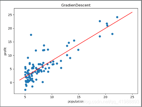
梯度下降法
import numpy as np
import pandas as pd
import matplotlib.pyplot as plt
def CostFunction(x,y,theta):
return np.sum((x.dot(theta) - y)**2) / (2 * len(x))
def GradienDescent(x,y,theta):
cost=[]
a=0.01
epcho=10000
for i in range(epcho):
temp=theta-(x.dot(theta)-y).dot(x)*a/(len(x))
theta=temp
#print("第",i+1,"次代价",CostFunction(x,y,theta))
cost.append(CostFunction(x,y,theta))
return theta,cost,epcho
f=open('ex1data1.txt',encoding='utf8')
data=pd.read_csv(f,header=None,names=['population','profit'])
x=data['population']
h=data['profit']
plt.scatter(x,h)
x = np.c_[np.ones(x.size), x]#详见机器学习(二)线性代数——计算技巧
theta=np.ones(x.shape[1])
theta,cost,epcho=GradienDescent(x,h,theta)
X=np.arange(4,25,0.01)
H=theta[0]+theta[1]*X
print(theta)
plt.title('GradienDescent')
plt.xlabel('population')
plt.ylabel('profit')
plt.plot(X,H,color='red')
plt.show()
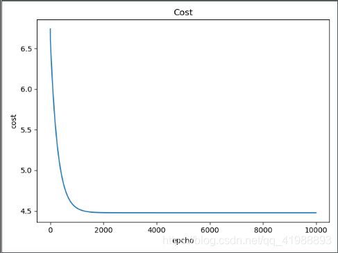
plt.xlabel('epcho')
plt.ylabel('cost')
plt.plot(range(epcho),cost)
plt.show()
#theta=[-3.89578081 1.19303364]
对上面第二个注释解释下:hypothesis: h(x)=0.5+40*x
x=[51213]
x=\left[
\begin{matrix}
5 \\
12 \\
13
\end{matrix}
\right]
x=⎣⎡51213⎦⎤
θ=[0.540]
θ=\left[
\begin{matrix}
0.5 \\
40
\end{matrix}
\right]
θ=[0.540]
通过那步变换,可以将x变为
x=[15112113]
x=\left[
\begin{matrix}
1&5 \\
1&12 \\
1&13
\end{matrix}
\right]
x=⎣⎡11151213⎦⎤
从而
h(x)=[1∗0.5+5∗401∗0.5+12∗401∗0.5+13∗40]
h(x)=\left[
\begin{matrix}
1*0.5+5*40\\
1*0.5+12*40\\
1*0.5+13*40
\end{matrix}
\right]
h(x)=⎣⎡1∗0.5+5∗401∗0.5+12∗401∗0.5+13∗40⎦⎤
使运算简便
结果如下:
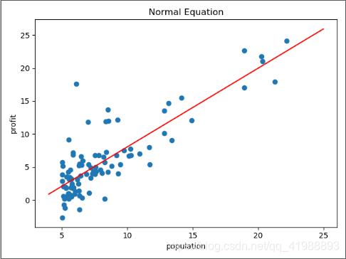
正规方程法
import numpy as np
import pandas as pd
import matplotlib.pyplot as plt
def LoadData():
    f=open('ex1data1.txt',encoding='utf8')
    data=pd.read_csv(f,header=None,names=['population','profit'])
    t=data['population']
    h=data['profit']
    x = np.c_[np.ones(t.size), t]
    return t,x,h
def NormalEquation(x,h):
    return ((np.linalg.inv((x.T).dot(x))).dot(x.T)).dot(h)
def main():
    t,x,h=LoadData()
    theta=NormalEquation(x,h)
    X=np.arange(4,25,0.01)
    H=theta[0]+theta[1]*X
    print(theta)
    plt.title('Normal Equation')
    plt.xlabel('population')
    plt.ylabel('profit')
    plt.scatter(t,h)
    plt.plot(X,H,color='red')
    plt.show()
if __name__ == '__main__':
    main()
    #theta=[-3.89578088  1.19303364]
结果如下:
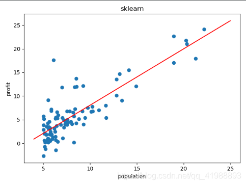
sklearn检验
import numpy as np
import pandas as pd
import matplotlib.pyplot as plt
from sklearn import linear_model
f=open('ex1data1.txt',encoding='utf8')
data=pd.read_csv(f,names=['population','profit'])
x=np.array(data['population']).reshape(-1,1)
y=np.array(data['profit']).reshape(-1,1)
plt.scatter(x,y)
model=linear_model.LinearRegression()
model.fit(x,y)
X=np.arange(4,25,0.01).reshape(-1,1)
H=model.predict(X)
plt.plot(X,H,color='red')
plt.show()
print(model.coef_)
print(model.intercept_)
结果如下:
斜率:1.19303364
截距:-3.89578088


 1272
1272

 被折叠的 条评论
为什么被折叠?
被折叠的 条评论
为什么被折叠?
 到【灌水乐园】发言


