Seurat-单细胞文献复现第二弹-01

最新推荐文章于 2024-07-31 01:22:04 发布

TTS56

最新推荐文章于 2024-07-31 01:22:04 发布

阅读量4.4k

点赞数 8

CC 4.0 BY-SA版权

分类专栏： CNS复现文章标签： r语言

本文链接：https://blog.youkuaiyun.com/qq_40966210/article/details/120758445

CNS复现专栏收录该内容

6 篇文章

订阅专栏

A single-cell map of intratumoral changes during anti-PD1 treatment of patients with breast cancer

https://doi.org/10.1038/s41591-021-01323-8

文章目录

A single-cell map of intratumoral changes during anti-PD1 treatment of patients with breast cancer
前言
讲在前面的废话
文章导读
图表复现

前言

Seurat-单细胞文献复现第二弹-01
Seurat-单细胞文献复现第二弹-02

讲在前面的废话

文章是一个好文章，但是没给代码，这一点就要差评

文章导读

Motivation：

To understand why only a subset of tumors respond to ICB（想了解一下免疫治疗耐受的原因）

Data：

one cohort of patients with non-metastatic, treatment-naive primary invasive carcinoma of the breast was treated with one dose of pembrolizumab (Keytruda or anti-PD1) approximately 9 ± 2 days before surgery (Fig. 1a and Methods). A second cohort of patients received neoadjuvant che- motherapy for 20–24 weeks, which was followed by pembrolizumab before surgery.
（一共两个队列，都是配套的数据，PD-L1 治疗前后的单细胞测序和 TCR）

图表复现

fig1 和配套的补充材料

Step.00 Download_Data

数据太大了，没办法从头处理，只能直接使用文献提供的数据，因为提供的是 rds 的文件，所以需要一些处理

a download of the read count data per individual patient
is publicly available at
http://biokey.lambrechtslab.org.

Convert sparse matrix to count matrix

# optionss
rm(list=ls())
gc()
options(stringsAsFactors = F)
options(as.is = T)

# packages
library(stringr)
library(magrittr)
library(Seurat)

# my_function
as_matrix <- function(mat){
  
  tmp <- matrix(data=0L, nrow = mat@Dim[1], ncol = mat@Dim[2])
  
  row_pos <- mat@i+1
  col_pos <- findInterval(seq(mat@x)-1,mat@p[-1])+1
  val <- mat@x
  
  for (i in seq_along(val)){
    tmp[row_pos[i],col_pos[i]] <- val[i]
  }
  
  row.names(tmp) <- mat@Dimnames[[1]]
  colnames(tmp) <- mat@Dimnames[[2]]
  return(tmp)
}

# load data
if(F){
  cohort1 = readRDS("../rawdata/1863-counts_cells_cohort1.rds")
  df1 = as_matrix(cohort1)
  cohort2 = readRDS("../rawdata/1867-counts_cells_cohort2.rds")
  df2 = as_matrix(cohort2)
  save(df1,df2,file = '../rawdata/cohort1_and_cohort2.rdata')
}

首先第一步就是获取 Seurat 对象，这一部分文章只用了 cohor1的队列

Step.01 Create Seurat obj for Cohort1

# options
rm(list=ls())
gc()
options(stringsAsFactors = F)
options(as.is = T)

# packages 
library(stringr)
library(magrittr)
library(Seurat)

# set work-dir
setwd('/Yours')

# load data 
load("Count/cohort1_and_cohort2.rdata")
predict = read.csv('output/raw_predict-Cohort1.csv',row.names = 1)
meta = read.csv('Count/1872-BIOKEY_metaData_cohort1_web.csv',row.names = 1)
rm(df2)
gc()
ids = predict %>% rownames()
meta$CellType = ifelse(rownames(meta) %in% ids,predict$label,meta$cellType)

# Create Seurat obj
sce = CreateSeuratObject(counts = df1)
sce = AddMetaData(sce, metadata = meta)
save(sce,file='output/cohort1_sce.rdata')

Step.02 Data clean & Standerdize processing

根据文章在 Method 中的信息进行数据处理

All cells expressing <200 or >6,000 genes were removed, as well as cells that contained <400 unique molecular identifiers (UMIs) and >15% mitochondrial counts.

数据中是没有 UMI 信息的

# options
rm(list=ls())
gc()
options(stringsAsFactors = F)
options(as.is = T)

# packages 
library(stringr)
library(magrittr)
library(Seurat)

# set work-dir
setwd('/Yours')

# load data 
load('output/cohort1_sce.rdata')
tcr = read.csv('scTCR/1879-BIOKEY_barcodes_vdj_combined_cohort1.csv')
tcr.info = read.csv('scTCR/1881-BIOKEY_clonotypes_combined_cohort1.csv')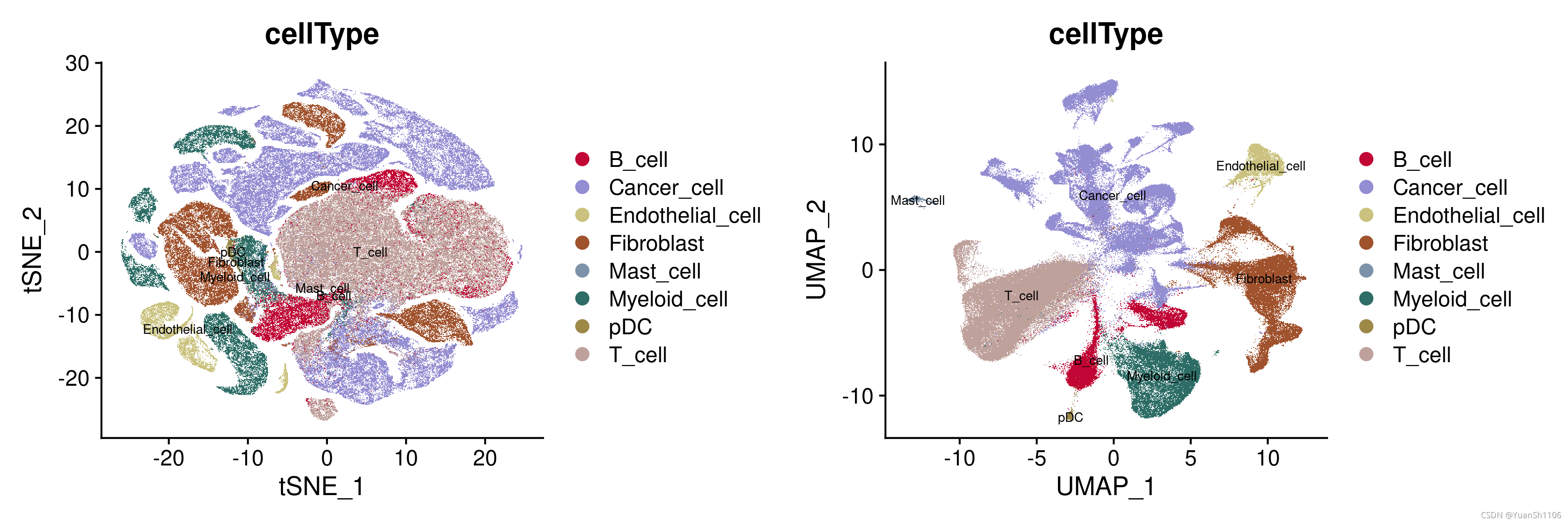![请添加图片描述](https://img-blog.csdnimg.cn/323c827b6a8243dd98dd6a5e1816ad68.png?x-oss-process=image/watermark,type_ZHJvaWRzYW5zZmFsbGJhY2s,shadow_50,text_Q1NETiBAWXVhblNoMTEwNg==,size_20,color_FFFFFF,t_70,g_se,x_16)

# my functions 
# mycolors = stata_pal("s2color")(15)
mycolors = c("#1a476f","#90353b","#55752f","#e37e00","#6e8e84",
             "#c10534","#938dd2","#cac27e","#a0522d","#7b92a8",
             "#2d6d66","#9c8847","#bfa19c","#ffd200","#d9e6eb")
             
# clean 
# 1. All cells expressing <200 or >6,000 genes
# 2. <400 unique molecular identifiers (UMIs)
# 3. >15% mitochondrial counts.
mt = grep('^MT-', x= rownames(sce),value = T) 
sce[["percent.mt"]]  = PercentageFeatureSet(sce, pattern = "^MT-")

# 1.log
sce = NormalizeData(object = sce,normalization.method =  "LogNormalize",  scale.factor = 1e4)
# 2.FindVariable
sce = FindVariableFeatures(object = sce,selection.method = "vst", nfeatures = 2000)
# 3.ScaleData
sce = ScaleData(object = sce)
# 4. PCA
sce = RunPCA(object = sce, do.print = FALSE)
# 5.Neighbor
sce= FindNeighbors(sce, dims = 1:20)
# 6. Clusters
sce = FindClusters(sce, resolution = 0.5) 
# 7.tsne
sce=RunTSNE(sce,dims.use = 1:20)
# 8.plot
p1 = DimPlot(sce,reduction = "tsne",label=T, group.by = "cellType",cols=mycolors[6:15],label.size=2.5)
p2 = DimPlot(sce,reduction = "umap",label=T, group.by = "cellType",cols=mycolors[6:15],label.size=2.5)
CombinePlots(plots =list(p1, p2))
ggsave('plot/Cohort1_CellType_plot.png', width = 12, height = 4)

经过检查发现数据是经过过滤的，所以不需要进行过滤操作，直接跑流程就行。

由于文章没有给出明确的参数，所以这里只能按照标准流程跑了

分群后使用原文的标签进行可视化评估，从图中可以看出来，分群的结果还可以（UMAP），各个细胞的分群边界比较清晰。

验证一下原始文献的注释结果，从UMAP的结果可以看出，不同的细胞类型离散程度较高

Step.03 Cell Annotion

根据文章补充材料的基因 marker 进行注释。
有一点值得注意一下，
这篇文章不是根据 epcam 进行肿瘤细胞定义的，然后我自己去用 epcam 评估过后发现这部分的 epcam 表达丰度很低
并且使用 BscModel 评估后发现，这部分的肿瘤候选细胞纯度很高，还是比较可信的

Next, we annotate cells using genes in artical

# get gene list 
gene.list = c('CD3D','CD3E','CD2',
              'COL1A1','DCN','C1R',
              'LYZ','CD68','TYROBP',
              'CD24','KRT19','SCGB2A2',
              'CD79A','MZB1','MS4A1',
              'CLDN5','FLT1','RAMP2',
              'CPA3','TPSAB1','TPSB2',
              'LILRA4','CXCR3','IRF7')
FeaturePlot(object = sce, features=gene.list)
p = DotPlot(sce, features = gene.list) + coord_flip()
p
ggsave('plot/Cell_annotion_DotPlot.png', width = 10, height = 10)

细胞群落的基因表达丰度图

根据原文的基因集，查看不同细胞群落的特意基因表达情况

细胞注释流程

由于这部分的细胞分群太多，而且基因也很多，一个个看过去眼睛会瞎掉，所以先进行粗注释然后在进行细注释

### Cell Markers
T.cell.marker = c("CD3D",'CD3E','CD2')
Fib.cell.marker = c('COL1A1','DCN','C1R')
Myeioid.cell.marker = c('LYZ','CD68','TYROBP')
Cancer.cell.marker = c('CD24','KRT19','SCGB2A2')
B.cell.marker= c('CD79A','MZB1','MS4A1')
Endothelial.cell.marker= c('CLDN5','FLT1','RAMP2')
Mast.cell.marker= c('CPA3','TPSAB1','TPSB2')
DC.cell.marker= c('LILRA4','CXCR3','IRF7')

### Define CellType
cell_type = c('T-cell','Fibroblast','Myeloid cell','Cancer cell','B-cell','Endothelial cell','Mast cell',"pDC")
markers = c("T.cell.marker","Fib.cell.marker","Myeioid.cell.marker","Cancer.cell.marker", "B.cell.marker","Endothelial.cell.marker", "Mast.cell.marker","DC.cell.marker")



# Cell types were preliminarily identified according to expression levels
for(i in 1:length(cell_type)){
  p = DotPlot(sce, features = get(markers[i])) + coord_flip()
  ids = as.numeric(p$data[which(p$data$avg.exp.scaled > 0 ),]$id)-1
  ids = table(ids)[which(table(ids) >=2)] %>% names() %>% as.numeric()
  ids = rownames(sce@meta.data[which(sce@meta.data$seurat_clusters %in% ids),])
  assign(cell_type[i], ids)
}
length(c(get(cell_type[1]),get(cell_type[2]),get(cell_type[3]),get(cell_type[4]),get(cell_type[5]),get(cell_type[6]),get(cell_type[7]),get(cell_type[8])))
ids = unique(c(get(cell_type[1]),get(cell_type[2]),get(cell_type[3]),get(cell_type[4]),get(cell_type[5]),get(cell_type[6]),get(cell_type[7]),get(cell_type[8])))
rest = setdiff(rownames(sce@meta.data),ids)
sce@meta.data$cell_annotion = ifelse(rownames(sce@meta.data) %in% get(cell_type[1]),cell_type[1],
                                     ifelse(rownames(sce@meta.data) %in% get(cell_type[2]),cell_type[2],
                                            ifelse(rownames(sce@meta.data) %in% get(cell_type[3]),cell_type[3],
                                                   ifelse(rownames(sce@meta.data) %in% get(cell_type[4]),cell_type[4],
                                                          ifelse(rownames(sce@meta.data) %in% get(cell_type[5]),cell_type[5],
                                                                 ifelse(rownames(sce@meta.data) %in% get(cell_type[6]),cell_type[6],
                                                                        ifelse(rownames(sce@meta.data) %in% get(cell_type[7]),cell_type[7],
                                                                               ifelse(rownames(sce@meta.data) %in% get(cell_type[8]),cell_type[8],'rest'))))))))


### Check Unique & consistency
check.unique = NULL
for(i in 1:7){
  for(j in (i+1):8){
    len = intersect(get(cell_type[i]),get(cell_type[j]))
    if(length(len) != 0 ){
      ids = c(cell_type[i],cell_type[j],markers[i],markers[j],length(len))
      check.unique = rbind(check.unique,ids)
    }
  }
}
check.unique


##### Manual Adjust
i=5 # for i in 1:dim(check.unique)[1]
ids1 = check.unique[i,1]
ids2 = check.unique[i,2]
gen1 = check.unique[i,3]
gen2 = check.unique[i,4]
ids = intersect(get(ids1),get(ids2))
DotPlot(sce[,ids], features = c(get(gen1),get(gen2)))  + coord_flip()
ids1
ids2
DotPlot(sce[,rest], features =gene.list)  + coord_flip()
DotPlot(sce, features =c(get('B.cell.marker'),get('Cancer.cell.marker')))   + coord_flip()

sce@meta.data[which(sce@meta.data$seurat_clusters == 19),'cell_annotion'] = "T-cell"
sce@meta.data[which(sce@meta.data$seurat_clusters == 1),'cell_annotion'] = "T-cell"
sce@meta.data[which(sce@meta.data$seurat_clusters == 6),'cell_annotion'] = "T-cell"
sce@meta.data[which(sce@meta.data$seurat_clusters == 33),'cell_annotion'] = "Fibroblast"
sce@meta.data[which(sce@meta.data$seurat_clusters == 30),'cell_annotion'] = "Fibroblast"
sce@meta.data[which(sce@meta.data$seurat_clusters == 8),'cell_annotion'] = "Cancer cell"
sce@meta.data[which(sce@meta.data$seurat_clusters == 23),'cell_annotion'] = "Cancer cell"
sce@meta.data[which(sce@meta.data$seurat_clusters == 24),'cell_annotion'] = "Cancer cell"
sce@meta.data[which(sce@meta.data$seurat_clusters == 18),'cell_annotion'] = "Cancer cell"
sce@meta.data[which(sce@meta.data$seurat_clusters == 29),'cell_annotion'] = "pDC"

##### consistency
sce@meta.data$cell_annotion = str_replace_all(sce@meta.data$cell_annotion, c("B-cell" = "B_cell",
                                               "Cancer cell" = "Cancer_cell",
                                               "Endothelial cell" = "Endothelial_cell",
                                               "Fibroblast" = "Fibroblast",
                                               "Mast cell" = "Mast_cell",
                                               "Myeloid cell" = "Myeloid_cell",
                                               "pDC" = "pDC",
                                               "T-cell" = "T_cell"))

### plot
p1 = DimPlot(sce,reduction = "tsne",label=T, group.by = "cell_annotion",cols=mycolors[6:15],label.size=2.5)
p2 = DimPlot(sce,reduction = "umap",label=T, group.by = "cell_annotion",cols=mycolors[6:15],label.size=2.5)
CombinePlots(plots =list(p1, p2))
ggsave('plot/Cohort1_cell_annotion_plot.png', width = 12, height = 4)

自己的分群结果，与原文的一致性97.26%

Marker gene 热图

### plot
p1 = DimPlot(sce,reduction = "tsne",label=T, group.by = "cell_annotion",cols=mycolors[6:15],label.size=2.5)
p2 = DimPlot(sce,reduction = "umap",label=T, group.by = "cell_annotion",cols=mycolors[6:15],label.size=2.5)
CombinePlots(plots =list(p1, p2))
ggsave('plot/Cohort1_cell_annotion_plot.png', width = 12, height = 4)

# cell type heat-map
for(i in 1:length(gene.list)){
  ids = sce[gene.list[i],]
  ids = ids@assays$RNA@data %>% as.numeric()
  assign(gene.list[i],tapply(ids, sce@meta.data$cell_annotion,mean))
}

heatmap_matrix = NULL
for (i in 1:length(gene.list)) {
  heatmap_matrix = rbind(heatmap_matrix,get(gene.list[i]))
}
row.names(heatmap_matrix) = gene.list
ids = c("T_cell","Fibroblast","Myeloid_cell","Cancer_cell","B_cell","Endothelial_cell","Mast_cell","pDC")
heatmap_matrix = heatmap_matrix[,ids]
pheatmap::pheatmap(heatmap_matrix,scale = 'row',cluster_cols = F,cluster_rows = F,filename = 'plot/Cohort1_cell_annotion_hm.png')
meta = sce@meta.data

这个和原文基本上完全一样，可以自行对比

治疗前后细胞比例变化

# NE / E 
names(table(meta$patient_id))
ids = c(7,9,18,20,4,13,19,22,23,26,29,30,21,28,31,11,5,17,27,6,12,16,10,3,8,25,14,24,2)
ids = paste0('BIOKEY','_',ids)
meta = meta[which(meta$patient_id %in% ids),]
E = c('BIOKEY_12','BIOKEY_16','BIOKEY_10','BIOKEY_3','BIOKEY_8','BIOKEY_25','BIOKEY_14','BIOKEY_24','BIOKEY_2')
meta$Ne_type = ifelse(meta$patient_id %in% E,'E','NEs')

# pre- / on- cell rations
pre = meta[which(meta$timepoint == 'Pre'),]
on = meta[which(meta$timepoint == 'On'),]
ids1 = table(pre$cell_annotion) %>% as.data.frame()
ids2 = table(on$cell_annotion) %>% as.data.frame()
ids1$group = 'pre'
ids2$group = 'on'
df = rbind(ids1,ids2)

ggplot(data=df, mapping=aes(x=Freq,y=Var1,fill=group))+
  geom_bar(stat='identity',width=0.5,position='fill')+theme_bw()+scale_fill_manual(values = mycolors[7:6])+geom_vline(aes(xintercept=0.48),color = 'black',linetype='dashed')
ggsave('plot/Cohort1_cell_ratio_bar_plot.png', width = 6.7, height = 7.6)

请添加图片描述

NE / Es 的变化

df = pre
ids = table(df$patient_id) %>% as.data.frame()
df.plot = table(df[,c('patient_id','cell_annotion')]) %>% as.data.frame()
df.plot$prop = 0
for(i in 1:dim(ids)[1]){
  prop.temp = df.plot[which(df.plot$patient_id %in% ids[i,1]),'Freq'] / ids[i,2]
  df.plot[which(df.plot$patient_id %in% ids[i,1]),'prop'] = prop.temp
}
df.plot$cell_annotion = factor(df.plot$cell_annotion,levels = c("T_cell","Fibroblast","Myeloid_cell","Cancer_cell","B_cell","Endothelial_cell","Mast_cell","pDC"))
df.plot$Ne_type = ifelse(df.plot$patient_id %in% E,'E','NEs')
df.plot$Ne_type = factor(df.plot$Ne_type,levels = c('NEs','E'))
df.plot
ggplot(data=df.plot, mapping=aes(x=cell_annotion,y=prop,color=Ne_type))+
  geom_boxplot()+theme_bw()+scale_color_manual(values = mycolors[7:6])
ggsave('plot/Cohort1_pre_box_plot.png', width = 8.24, height = 2.84)

df = on
ids = table(df$patient_id) %>% as.data.frame()
df.plot = table(df[,c('patient_id','cell_annotion')]) %>% as.data.frame()
df.plot$prop = 0
for(i in 1:dim(ids)[1]){
  prop.temp = df.plot[which(df.plot$patient_id %in% ids[i,1]),'Freq'] / ids[i,2]
  df.plot[which(df.plot$patient_id %in% ids[i,1]),'prop'] = prop.temp
}
df.plot$cell_annotion = factor(df.plot$cell_annotion,levels = c("T_cell","Fibroblast","Myeloid_cell","Cancer_cell","B_cell","Endothelial_cell","Mast_cell","pDC"))
df.plot$Ne_type = ifelse(df.plot$patient_id %in% E,'E','NEs')
df.plot$Ne_type = factor(df.plot$Ne_type,levels = c('NEs','E'))
df.plot
ggplot(data=df.plot, mapping=aes(x=cell_annotion,y=prop,color=Ne_type))+
  geom_boxplot()+theme_bw()+scale_color_manual(values = mycolors[7:6])
ggsave('plot/Cohort1_on_box_plot.png', width = 8.24, height = 2.84)

请添加图片描述

Step.04 Cancer cell detection

BscModel

First, get logNormalize data and the follow the document of BscModel to set config

# cohort1
sce = CreateSeuratObject(counts = df1)
sce = AddMetaData(sce, metadata = sd1)
sce <- NormalizeData(object = sce, scale.factor = 1e6)
use.cells = sce@meta.data[which(sce@meta.data$cellType == 'Cancer_cell'),] %>% rownames()
sce = subset(sce,cells = use.cells)
df = sce@assays$RNA@data %>% as.data.frame()
max(df)
min(df)
write.csv(df,'../processfile/Cohort1_epi_expr.csv')

# cohort2
sce = CreateSeuratObject(counts = df2)
sce = AddMetaData(sce, metadata = sd2)
sce <- NormalizeData(object = sce, scale.factor = 1e6)
use.cells = sce@meta.data[which(sce@meta.data$cellType == 'Cancer_cell'),] %>% rownames()
sce = subset(sce,cells = use.cells)
df = sce@assays$RNA@data %>% as.data.frame()
max(df)
min(df)
write.csv(df,'../processfile/Cohort2_epi_expr.csv')

Then, run the script

python main.py --config configs/Training_and_predict.yaml

InferCNV

Prepare file & Run

# main 
# 导入原始表达矩阵
# main 
# 导入原始表达矩阵
if(T){
  load("./rawdata/cohort1_and_cohort2.rdata")
  rm(df2)
  gc()
  info = read.csv('processfile/predict-Cohort1.csv',row.names = 1)
  info = info[which(info$label!='Moderate'),]
  #use.cell = info$X
  meta = read.csv('rawdata/1872-BIOKEY_metaData_cohort1_web.csv',row.names = 1)
  meta$cellType = ifelse(rownames(meta) %in% rownames(info),info$label,meta$cellType)
}
meta[which(meta$cellType == 'Cancer_cell'),'cellType'] = 'Moderate'
info = meta
a = names(table(info$cellType))
for(i in a){print(i)}

use.cell = c("Endothelial_cell",
             "Fibroblast",
             "Moderate",
             "Normal",
             "Tumor")

use.cell = c("B_cell",
             "Mast_cell",
             "Moderate",
             "Myeloid_cell",
             "Normal",
             "pDC",
             "T_cell",
             "Tumor")
use.cell = info[which(info$cellType %in% use.cell),] %>% rownames()
#df2 = df2[,use.cell]
df1 = df1[,use.cell]
info = info[use.cell,]

if(T){
  # 第一个文件count矩阵
  dfcount = df1
  # 第二个文件样本信息矩阵
  groupinfo= data.frame(cellId = colnames(dfcount))
  identical(groupinfo[,1],rownames(info))
  groupinfo$cellType = info$cellType
  
  # 第三文件
  library(AnnoProbe)
  geneInfor=annoGene(rownames(dfcount),"SYMBOL",'human')
  geneInfor=geneInfor[with(geneInfor, order(chr, start)),c(1,4:6)]
  geneInfor=geneInfor[!duplicated(geneInfor[,1]),]
  
  ## 这里可以去除性染色体
  # 也可以把染色体排序方式改变
  dfcount =dfcount [rownames(dfcount ) %in% geneInfor[,1],]
  dfcount =dfcount [match( geneInfor[,1], rownames(dfcount) ),] 
  
  myhead(dfcount)
  myhead(geneInfor)
  myhead(groupinfo)
  # 输出
  expFile='./processfile/88284_expFile.txt'
  write.table(dfcount ,file = expFile,sep = '\t',quote = F)
  groupFiles='./processfile/88284_groupFiles.txt'
  write.table(groupinfo,file = groupFiles,sep = '\t',quote = F,col.names = F,row.names = F)
  geneFile='./processfile/88284_geneFile.txt'
  write.table(geneInfor,file = geneFile,sep = '\t',quote = F,col.names = F,row.names = F)
}
# infercnv流程
a = names(table(groupinfo$cellType))
for(i in a){print(i)}

if(T){
  rm(list=ls())
  setwd('/media/yuansh/14THHD/胶囊单细胞/测试集/EGAD/')
  options(stringsAsFactors = F)
  library(Seurat)
  library(ggplot2)
  library(infercnv)
  expFile='./processfile/88284_expFile.txt' 
  groupFiles='./processfile/88284_groupFiles.txt'  
  geneFile='./processfile/88284_geneFile.txt'
  library(infercnv)
  infercnv_obj = CreateInfercnvObject(raw_counts_matrix=expFile,
                                      annotations_file=groupFiles,
                                      delim="\t",
                                      gene_order_file= geneFile,
                                      ref_group_names=c("Endothelial_cell",
                                                        "Fibroblast")) # 如果有正常细胞的话，把正常细胞的分组填进去
  library(future)
  plan("multiprocess", workers = 16)
  infercnv_all = infercnv::run(infercnv_obj,
                               cutoff=0.1,  # use 1 for smart-seq, 0.1 for 10x-genomics
                               out_dir= "./processfile/88284_inferCNV_Cohort1",  # dir is auto-created for storing outputs
                               cluster_by_groups=T,   # cluster
                               num_threads=32,
                               denoise=F,
                               HMM=F)
}

请添加图片描述

这里展示的是 Cohort2 数据，因此图和原文有差异

### ---------------
###
### Create: Yuan.Sh
### Date: 2021-10-14 23:52:41
### Email: yuansh3354@163.com
### Blog: https://blog.youkuaiyun.com/qq_40966210
### Fujian Medical University
###
### ---------------

> 课题项目合作以及咨询请联系：yuansh3354@163.com

After advisement, if you still have questions, you can send me an E-mail asking for help
Best Regards,
Yuan.SH
---------------------------------------
please contact me via the following ways:
(a) E-mail: yuansh3354@gmail/163/outlook.com
(b) QQ: 1044532817
(c) WeChat: YuanSh181014
(d) Address: School of Basic Medical Sciences, 
Fujian Medical University, Fuzhou, 
Fujian 350108, China
---------------------------------------