


 本文详细介绍了深度神经网络的前向传播过程,包括训练单个样本时的计算步骤和向量化处理。在前向传播中,每个层的计算遵循z[l]=w[l]a[l−1]+b[l],a[l]=g[l](z[l])的规则。反向传播用于计算梯度,更新参数以减小损失函数。在多层神经网络中,前向传播和反向传播涉及到多个隐藏层的线性与非线性组合。最后,通过示例代码展示了如何实现和优化参数更新过程,以实现网络的训练和预测。
深层神经网络
深层神经网络中的前向传播

-
训练单个样本:
第一层:
z [ 1 ] = w [ 1 ] x + b [ 1 ] a [ 1 ] = g ( z [ 1 ] ) \begin{array}{l} {z^{[1]}} = {w^{[1]}}x + {b^{[1]}}\\ {a^{[1]}} = g({z^{[1]}}) \end{array} z[1]=w[1]x+b[1]a[1]=g(z[1])
输入特征向量x也是第0层的激活单元,即 a [ 0 ] a^{[0]} a[0]
第一个式子可以改写成
z [ 1 ] = w [ 1 ] a [ 0 ] + b [ 1 ] {z^{[1]}} = {w^{[1]}}{a^{[0]}} + {b^{[1]}} z[1]=w[1]a[0]+b[1]
第二层:
z [ 2 ] = w [ 2 ] a [ 1 ] + b [ 2 ] a [ 2 ] = g [ 2 ] ( z [ 2 ] ) \begin{array}{l} {z^{[2]}} = {w^{[2]}}{a^{[1]}} + {b^{[2]}}\\ {a^{[2]}} = {g^{[2]}}({z^{[2]}}) \end{array} z[2]=w[2]a[1]+b[2]a[2]=g[2](z[2])
以此类推…
第四层:
z [ 4 ] = w [ 4 ] a [ 3 ] + b [ 4 ] a [ 4 ] = g [ 4 ] ( z [ 4 ] ) = y ^ \begin{array}{l} {z^{[4]}} = {w^{[4]}}{a^{[3]}} + {b^{[4]}}\\ {a^{[4]}} = {g^{[4]}}({z^{[4]}}) = \hat y \end{array} z[4]=w[4]a[3]+b[4]a[4]=g[4](z[4])=y^
基本规律:
z [ l ] = w [ l ] a [ l − 1 ] + b [ l ] a [ l ] = g [ l ] ( z [ l ] ) \begin{array}{l} {z^{[l]}} = {w^{[l]}}{a^{[l - 1]}} + {b^{[l]}}\\ {a^{[l]}} = {g^{[l]}}({z^{[l]}}) \end{array} z[l]=w[l]a[l−1]+b[l]a[l]=g[l](z[l]) -
使用向量化的方法训练整个训练集:
Z [ 1 ] = w [ 1 ] A [ 0 ] + b [ 1 ] A [ 1 ] = g [ 1 ] ( Z [ 1 ] ) \begin{array}{l} {Z^{[1]}} = {w^{[1]}}A^{[0]} + {b^{[1]}}\\ {A^{[1]}} = {g^{[1]}}({Z^{[1]}}) \end{array} Z[1]=w[1]A[0]+b[1]A[1]=g[1](Z[1])
(其中 A [ 0 ] A^{[0]} A[0]为 X X X)
同理其它层
最后得到:
Y ^ = g ( Z [ 4 ] ) = A [ 4 ] \hat Y = g({Z^{[4]}}) = {A^{[4]}} Y^=g(Z[4])=A[4]
实际上运算的过程就是一个for循环,从第一层计算到第L层(输入层到输出层)。
在实现深度神经网络的过程中,提高得到没有bug的程序的概率的一个方法就是需要非常仔细和系统化地去思考矩阵的维数。
核对矩阵的维数

- 正向传播:
z [ 1 ] = w [ 1 ] x + b [ 1 ] {z^{[1]}} = {w^{[1]}}x + {b^{[1]}} z[1]=w[1]x+b[1]
暂时忽略偏置项b,只关注参数w
图中 n [ 0 ] = n x = 2 n^{[0]}=n_{x}=2 n[0]=nx=2、 n [ 1 ] = 3 n^{[1]}=3 n[1]=3、 n [ 2 ] = 5 n^{[2]}=5 n[2]=5、 n [ 3 ] = 4 n^{[3]}=4 n[3]=4、 n [ 4 ] = 2 n^{[4]}=2 n[4]=2、 n [ 5 ] = 1 n^{[5]}=1 n[5]=1
z [ 1 ] z^{[1]} z[1]是第一个隐层的激活函数向量,在这里z 的维度为 (3,1),即一个三维向量或是 ( n [ 1 ] n^{[1]} n[1],1)维向量。
x在这里有2个输入特征,所以x的维度是 (2,1),归纳来说x的维度是( n [ 0 ] n^{[0]} n[0],1)。
所以需要利用矩阵 w [ 1 ] w^{[1]} w[1]来实现这样的结果,在这里运用矩阵乘法可以得到w的维度为 (3,2),即 ( n [ 1 ] n^{[1]} n[1], n [ 0 ] n^{[0]} n[0]) - 归纳来说就是
w
l
w^{l}
wl的维度必须是 (
n
[
l
]
n^{[l]}
n[l],
n
[
l
−
1
]
n^{[l-1]}
n[l−1])。
b [ l ] b^{[l]} b[l]应该和 w [ l ] w^{[l]} w[l] a [ l − 1 ] a^{[l-1]} a[l−1]的维度相同,所以 b [ l ] b^{[l]} b[l]的维度应为 ( n [ l ] n^{[l]} n[l],1) - 当实现反向传播时,
d
w
[
l
]
dw^{[l]}
dw[l]的维度应和
w
[
l
]
w^{[l]}
w[l]的维度相同,即为 (
n
[
l
]
n^{[l]}
n[l],
n
[
l
−
1
]
n^{[l-1]}
n[l−1])
d b [ l ] db^{[l]} db[l]和 b [ l ] b^{[l]} b[l]同维度。
由于 a [ l ] = g [ l ] ( z [ l ] ) {a^{[l]}} = {g^{[l]}}({z^{[l]}}) a[l]=g[l](z[l]), a [ l ] a^{[l]} a[l]和 z [ l ] z^{[l]} z[l]维度相同
即使实现过程已经向量化了,w、b、dw、db的维度应该始终一样。但是z、a和x的维度会在向量后发生变化。 - 当有多个样本时,
Z
[
1
]
Z^{[1]}
Z[1]为每个单独的
z
[
1
]
z^{[1]}
z[1]的值叠加得到的,即
Z [ 1 ] = [ z [ 1 ] ( 1 ) , z [ 1 ] ( 2 ) , . . . , z [ 1 ] ( m ) ] {Z^{[1]}} = [{z^{[1](1)}},{z^{[1](2)}},...,{z^{[1]\left( m \right)}}] Z[1]=[z[1](1),z[1](2),...,z[1](m)]
维度为 ( n [ 1 ] , m ) (n^{[1]},m) (n[1],m),其中m是训练集的大小, W [ 1 ] W^{[1]} W[1]的维度不变 ( n [ 1 ] , n [ 0 ] ) (n^{[1]},n^{[0]}) (n[1],n[0]),X的维度为 ( n [ 0 ] , m ) (n^{[0]},m) (n[0],m), b [ 1 ] b^{[1]} b[1]维度不变 ( n [ 1 ] , 1 ) (n^{[1]},1) (n[1],1)。 - 归纳来说:
Z [ l ] , A [ l ] : ( n [ l ] , m ) Z^{[l]},A^{[l]}:(n^{[l]},m) Z[l],A[l]:(n[l],m)
d Z [ l ] , d A [ l ] : ( n [ l ] , m ) dZ^{[l]},dA^{[l]}:(n^{[l]},m) dZ[l],dA[l]:(n[l],m)
在写程序时,一定要确认所有的矩阵维数前后一致,可以很好的排除程序中的一些错误。
为什么需要深层表示
-
深度网络在计算什么
当输入一张脸部照片,可以把深度神经网络的第一层当成一个特城探测器,或是边缘探测器。
在这个例子中,将会建立一个约有20个隐藏单元的深度神经网络来对这张图进行计算。隐藏单元就是下图中的小方块,使用这些小方块来寻找照片中边缘的方向。

可以把照片中组成边缘的像素们放在一起查看,它可以把被检测到的边缘组合成面部的不同部分。如下图,比方说其中一个神经元用于检测眼睛,另一个神经元用于检测鼻子。将这些边缘结合在一起,就可以开始检测人脸的不同部分。

最后再将这些部分放在一起,就可以识别或是检测不同的人脸。

可以简单的把这种神经网络的前几层当做例如边缘检测的简单检测函数,再将它与后几层结合,就可以学习得到一个复杂的函数。
(边缘探测器其实相对来说都是针对照片中非常小块的面积,而面部探测器就会针对大一些的区域,是一种从简单到复杂的金字塔状表示方式\组成方式,这种方式还可以应用于除人脸识别或图像以外的其他数据上)
在深度神经网络的许多隐层中,前几层学习一些低层次的简单特征,后几层将简单的特征结合起来去探测更加复杂的东西。 -
为什么需要深层网络
这来源于电路理论,与可以使用哪些电路元件计算哪些函数有着分不开的联系,在一般情况下,这些函数都可以使用隐藏单元数量相对较少,但是很深的神经网络来计算。但是如果使用一些浅层的神经网络(隐藏层数少)来计算同样的函数,会需要呈指数增长的单元数量才能达到同样的计算结果。
深度学习实际上就是有很多隐藏层的神经网络。(但是面对实际问题处理时,并不需要一开始就建立很多隐藏层,先从logistic回归开始,再试着使用1到2个隐藏层,将隐层的数量当做参数或超参数一样去调试,找到合适的深度即可)
搭建深层神经网络块
- 正向反向传播函数

上图为一个层数较少的神经网络,选择框出来的一层,记这层为l层。
layer l: w [ l ] , b ( l ) w^{[l]},b^{(l)} w[l],b(l)
Forward:
input a [ l − 1 ] a^{[l-1]} a[l−1], output a [ l ] a^{[l]} a[l]
z [ l ] = w [ l ] a [ l − 1 ] + b [ l ] {z^{[l]}} = {w^{[l]}}a^{[l-1]} + {b^{[l]}} z[l]=w[l]a[l−1]+b[l]
a [ l ] = g [ l ] ( z [ l ] ) {a^{[l]}} = {g^{[l]}}({z^{[l]}}) a[l]=g[l](z[l])
这里要将 z [ l ] z^{[l]} z[l]缓存起来,因为它对之后的正向和反向传播都很有用
向量化:
Z [ l ] = W [ l ] A [ l − 1 ] + b [ l ] {Z^{[l]}} = {W^{[l]}}A^{[l-1]} + {b^{[l]}} Z[l]=W[l]A[l−1]+b[l]
A [ l ] = g [ l ] ( Z [ l ] ) {A^{[l]}} = {g^{[l]}}({Z^{[l]}}) A[l]=g[l](Z[l])
使用 X = A [ 0 ] X=A^{[0]} X=A[0]来初始化
Backward:input d a [ l ] da^{[l]} da[l]、 z [ l ] z^{[l]} z[l], output d a [ l − 1 ] da^{[l-1]} da[l−1]、 d w [ l ] dw^{[l]} dw[l]、 d b [ l ] db^{[l]} db[l]
d z [ l ] = d a [ l ] ∗ g [ l ] ′ ( z [ l ] ) dz^{[l]}=da^{[l]}*g^{[l]'}(z^{[l]}) dz[l]=da[l]∗g[l]′(z[l])
d w [ l ] = d z [ l ] ∗ a [ l − 1 ] dw^{[l]}=dz^{[l]}*a^{[l-1]} dw[l]=dz[l]∗a[l−1]
d b [ l ] = d z [ l ] db^{[l]}=dz^{[l]} db[l]=dz[l]
d a [ l − 1 ] = w [ l ] T ∗ d z [ l ] da^{[l-1]}=w^{[l]T}*dz^{[l]} da[l−1]=w[l]T∗dz[l]
d z [ l ] = w [ l + 1 ] T d z [ l + 1 ] ∗ g [ l ] ′ ( z [ l ] ) dz^{[l]}=w^{[l+1]T}dz^{[l+1]}*g^{[l]'}(z^{[l]}) dz[l]=w[l+1]Tdz[l+1]∗g[l]′(z[l])
向量化:
d Z [ l ] = d A [ l ] ∗ g [ l ] ′ ( Z [ l ] ) dZ^{[l]}=dA^{[l]}*g^{[l]'}(Z^{[l]}) dZ[l]=dA[l]∗g[l]′(Z[l])
d W [ l ] = 1 m d Z [ l ] ∗ A [ l − 1 ] T dW^{[l]}=\frac{1}{m}dZ^{[l]}*A^{[l-1]T} dW[l]=m1dZ[l]∗A[l−1]T
d b [ l ] = 1 m n p . s u m ( d z [ l ] , a x i s = 1 , k e e p d i m s = T r u e ) db^{[l]}=\frac{1}{m}np.sum(dz^{[l]},axis=1,keepdims=True) db[l]=m1np.sum(dz[l],axis=1,keepdims=True)
d A [ l − 1 ] = W [ l ] T ∗ d z [ l ] dA^{[l-1]}=W^{[l]T}*dz^{[l]} dA[l−1]=W[l]T∗dz[l]
 其中红色的箭头表示反向传播,指向方框的为输入,从方框指出的为输出,方框内为需要的参数,其中
d
z
[
l
]
dz^{[l]}
dz[l]需要计算。
其中红色的箭头表示反向传播,指向方框的为输入,从方框指出的为输出,方框内为需要的参数,其中
d
z
[
l
]
dz^{[l]}
dz[l]需要计算。
如果实现了正向传播和反向传播的函数,l层的神经网络的计算过程就会是下图所示: d
a
[
0
]
da^{[0]}
da[0]是输入特征的导数,没有用。
d
a
[
0
]
da^{[0]}
da[0]是输入特征的导数,没有用。
w和b在每一层被更新,α为学习率
w [ l ] : = w [ l ] − α d w [ l ] w^{[l]}:=w^{[l]}-\alpha dw^{[l]} w[l]:=w[l]−αdw[l]
b [ l ] : = b [ l ] − α d b [ l ] b^{[l]}:=b^{[l]}-\alpha db^{[l]} b[l]:=b[l]−αdb[l]
细节:将 z [ l ] {z^{[l]}} z[l]的值缓存下来,当编程实现时使用起来会很方便,便于反向传播中获取 w [ l ] , b ( l ) w^{[l]},b^{(l)} w[l],b(l),因为缓存了 z [ l ] {z^{[l]}} z[l]实际上也缓存了 w [ l ] , b ( l ) w^{[l]},b^{(l)} w[l],b(l),反向传播中直接将参数复制即可。
前向递归会用输入数据x来初始化。当使用Logistic回归做二分分类时反向递归时,
损失函数 L ( y ^ , y ) L(\hat y,y) L(y^,y)的导数等于 d a [ l ] = − y a + ( 1 − y ) ( 1 − a ) d{a^{[l]}} = - \frac{y}{a} + \frac{{(1 - y)}}{{(1 - a)}} da[l]=−ay+(1−a)(1−y)
向量化这个实现过程,初始化反向递归,
d A [ l ] = ( − y ( 1 ) a ( 1 ) + ( 1 − y ( 1 ) ) ( 1 − a ( 1 ) ) . . . − y ( m ) a ( m ) + ( 1 − y ( m ) ) ( 1 − a ( m ) ) ) d{A^{[l]}} = ( - \frac{{{y^{(1)}}}}{{{a^{(1)}}}} + \frac{{(1 - {y^{(1)}})}}{{(1 - {a^{(1)}})}}... - \frac{{{y^{(m)}}}}{{{a^{(m)}}}} + \frac{{(1 - {y^{(m)}})}}{{(1 - {a^{(m)}})}}) dA[l]=(−a(1)y(1)+(1−a(1))(1−y(1))...−a(m)y(m)+(1−a(m))(1−y(m)))
【机器学习里的复杂性是源于数据本身,而不是一行行的代码。】
参数vs超参数
之前的学习中用到的参数:
W
[
1
]
,
b
[
1
]
,
W
[
2
]
,
b
[
2
]
,
W
[
3
]
,
b
[
3
]
.
.
.
W^{[1]},b^{[1]},W^{[2]},b^{[2]},W^{[3]},b^{[3]}...
W[1],b[1],W[2],b[2],W[3],b[3]...
除此之外还有输入到学习算法中的:学习率α,梯度下降法循环的数量,隐层数L,隐藏单元数,激活函数类型或是其他需要设置的数字,这些参数控制了参数W和b,所以被称之为超参数。(深度学习中包含很多超参数,例如momentum,minibatch size,regularizations…)
一般情况的调参过程还是比较经验性的。先假设一个学习率,在实际训练查看其效果(查看损失函数J有没有下降),基于尝试在对它进行调整(是否损失函数发散、收敛在更高的位置、快速下降或收敛在更低的位置)。其他超参数,例如隐层的数量同样需要实际测试调整。
【建议:刚开始应用新问题时,去试一定范围的值看看其结果。而一直使用认为的最优参数,在过段时间可能也会发生改变(因为其跟数据,电脑硬件也有关系),所以需要经常试试不同的超参数,勤于检验结果,慢慢的就会对超参数数值的设定更加得心应手。尝试保留交叉检验或类似检验方法。】
【后话(吴恩达教授):虽然深度学习的确是个很好的工具,能学习到各种很灵活和复杂的函数,学习从x到y的映射。在监督学习中,学到输入到输出的映射,但是这种运算和人类大脑(神经元)的类比,在这个领域的早期,也许还值得一提,但现在这种类比已经逐渐过时。】
课后作业
- “cache”记录了正向传播单元的值,并将其传给了反向传播单元,因为在计算链式法则导数时,需要用到这些值。
- 神经网络的更深层通常比前面的层计算更复杂的输入特征。
- 并不是向量化后的L层神经网络就不需要在1,2,…,L层上面使用显示for循环了(或其他显示迭代循环)
-假设将节点数 n [ l ] n^{[l]} n[l]的值存储在一个名为层的数组中,并且layer_dims=[n_x, 4, 3, 2, 1]。可以看到第一层有4个隐藏节点,第二层有3个隐藏节点…。如何使用for循环来初始化模型的参数。
# import numpy as np
# parameter = {}
# n_x = 10
# layer_dims = [n_x,4,3,2,1]
for i in range(1, len(layer_dims)):
    parameter['W' + str(i)] = np.random.randn(layer_dims[i],layer_dims[i-1]) * 0.01
    parameter['b' + str(i)] = np.random.randn(layer_dims[i],1) * 0.01
# print(parameter)
numpy.random.randn(d0, d1, …, dn) 是从标准正态分布中返回一个或多个样本值。
numpy.random.rand(d0, d1, …, dn) 的随机样本位于[0, 1)中。
基于numpy.random.randn()与rand()的区别详解
- 神经网络层数 = 隐藏层数 + 1
- 在前向传播中,需要记录每一层的激活函数,当反向传播时,需要用到一致的激活函数来完成梯度下降的导数计算。
假设输入数据X的维度为(12288,209)
| 层 | W的维度 | b的维度 | 激活值的计算 | 激活值的维度 |
|---|---|---|---|---|
| 第 1 层 | ( n [ 1 ] , 12288 ) (n^{[1]},12288) (n[1],12288) | ( n [ 1 ] , 1 ) (n^{[1]},1) (n[1],1) | Z [ 1 ] = W [ 1 ] X + b [ 1 ] Z^{[1]} = W^{[1]} X + b^{[1]} Z[1]=W[1]X+b[1] | ( n [ 1 ] , 209 ) (n^{[1]},209) (n[1],209) |
| 第 2 层 | ( n [ 2 ] , n [ 1 ] ) (n^{[2]}, n^{[1]}) (n[2],n[1]) | ( n [ 2 ] , 1 ) (n^{[2]},1) (n[2],1) | Z [ 2 ] = W [ 2 ] A [ 1 ] + b [ 2 ] Z^{[2]} = W^{[2]} A^{[1]} + b^{[2]} Z[2]=W[2]A[1]+b[2] | ( n [ 2 ] , 209 ) (n^{[2]}, 209) (n[2],209) |
| ⋮ \vdots ⋮ | ⋮ \vdots ⋮ | ⋮ \vdots ⋮ | ⋮ \vdots ⋮ | ⋮ \vdots ⋮ |
| 第 L-1 层 | ( n [ L − 1 ] , n [ L − 2 ] ) (n^{[L-1]},n^{[L-2]}) (n[L−1],n[L−2]) | ( n [ L − 1 ] , 1 ) (n^{[L-1]}, 1) (n[L−1],1) | Z [ L − 1 ] = W [ L − 1 ] A [ L − 2 ] + b [ L − 1 ] Z^{[L-1]}=W^{[L-1]}A^{[L-2]}+b^{[L-1]} Z[L−1]=W[L−1]A[L−2]+b[L−1] | ( n [ L − 1 ] , 209 ) (n^{[L-1]}, 209) (n[L−1],209) |
| 第 L 层 | ( n [ L ] , n [ L − 1 ] ) (n^{[L]}, n^{[L-1]}) (n[L],n[L−1]) | ( n [ L ] , 1 ) (n^{[L]}, 1) (n[L],1) | Z [ L ] = W [ L ] A [ L − 1 ] + b [ L ] Z^{[L]} = W^{[L]} A^{[L-1]} + b^{[L]} Z[L]=W[L]A[L−1]+b[L] | ( n [ L ] , 209 ) (n^{[L]}, 209) (n[L],209) |
- 使用np.sqrt(layers_dims[l - 1])是为了防止梯度爆炸与梯度消失的问题
详解深度学习中的梯度消失、爆炸原因及其解决方法 - python中np.multiply()、np.dot()和星号(*)三种乘法运算的区别
np.multiply():数组、矩阵对应位置元素相乘
np.sum():数组全部元素求和
np.mat():将数组转换为矩阵
np.dot():对于秩为1的数组,执行对应位置相乘,然后再相加;对于秩不为1的二维数组,执行矩阵乘法运算。
星号乘法(*):对数组执行对应位置相乘,对矩阵执行矩阵乘法运算。 - numpy.squeeze()的用法
从数组的形状中删除单维条目,即把shape中为1的维度去掉。 - keepdims主要用于保持矩阵的二维特性
array([[3], [7]])【keepdims=True】
array([3, 7]) - 元组赋值
In : a = [1,2,3]
In : b = [4,5,6]
In : c = [7,8,9]
In : d=(a,b,c)
In : q,w,e = d
In : q
Out : [1, 2, 3]
In : w
Out : [4, 5, 6]
In : e
Out : [7, 8, 9]
# 变量数超过元组中元素或少于元组中元素均不能赋值
- np.divide:数组对应位置元素做除法(非地板除)
- reversed 函数返回一个反转的迭代器。
# range仍然左闭右开
for i in reversed(range(3)):
    print(i)
out :
2
1
0
z = np.array([[1, 2, 3, 4],
          [5, 6, 7, 8],
          [9, 10, 11, 12],
          [13, 14, 15, 16]])
z.shape
(4, 4)
z.reshape(-1)
array([ 1,  2,  3,  4,  5,  6,  7,  8,  9, 10, 11, 12, 13, 14, 15, 16])
# 先前不知道z的shape属性是多少,但是想让z变成只有1列,行数不知道多少,通过`z.reshape(-1,1)`
z.reshape(-1,1)
 array([[ 1],
        [ 2],
        [ 3],
        [ 4],
        [ 5],
        [ 6],
        [ 7],
        [ 8],
        [ 9],
        [10],
        [11],
        [12],
        [13],
        [14],
        [15],
        [16]])
两层神经网络
import numpy as np
import h5py
import matplotlib.pyplot as plt
import testCases #参见资料包,或者在文章底部copy
from dnn_utils import sigmoid, sigmoid_backward, relu, relu_backward #参见资料包
import lr_utils #参见资料包,或者在文章底部copy
np.random.seed(1)
def initialize_parameters_deep(layers_dims):
"""
此函数是为了初始化多层网络参数而使用的函数。
参数:
layers_dims - 包含我们网络中每个图层的节点数量的列表
返回:
parameters - 包含参数“W1”,“b1”,...,“WL”,“bL”的字典:
W1 - 权重矩阵,维度为(layers_dims [1],layers_dims [1-1])
bl - 偏向量,维度为(layers_dims [1],1)
"""
np.random.seed(3)
parameters = {}
L = len(layers_dims)
for l in range(1,L):
parameters["W" + str(l)] = np.random.randn(layers_dims[l], layers_dims[l - 1]) / np.sqrt(layers_dims[l - 1])
parameters["b" + str(l)] = np.zeros((layers_dims[l], 1))
#确保我要的数据的格式是正确的
assert(parameters["W" + str(l)].shape == (layers_dims[l], layers_dims[l-1]))
assert(parameters["b" + str(l)].shape == (layers_dims[l], 1))
return parameters
def linear_forward(A,W,b):
"""
实现前向传播的线性部分。
参数:
A - 来自上一层(或输入数据)的激活,维度为(上一层的节点数量,示例的数量)
W - 权重矩阵,numpy数组,维度为(当前图层的节点数量,前一图层的节点数量)
b - 偏向量,numpy向量,维度为(当前图层节点数量,1)
返回:
Z - 激活功能的输入,也称为预激活参数
cache - 一个包含“A”,“W”和“b”的字典,存储这些变量以有效地计算后向传递
"""
Z = np.dot(W,A) + b
assert(Z.shape == (W.shape[0],A.shape[1]))
cache = (A,W,b)
return Z,cache
def linear_activation_forward(A_prev,W,b,activation):
"""
实现LINEAR-> ACTIVATION 这一层的前向传播
参数:
A_prev - 来自上一层(或输入层)的激活,维度为(上一层的节点数量,示例数)
W - 权重矩阵,numpy数组,维度为(当前层的节点数量,前一层的大小)
b - 偏向量,numpy阵列,维度为(当前层的节点数量,1)
activation - 选择在此层中使用的激活函数名,字符串类型,【"sigmoid" | "relu"】
返回:
A - 激活函数的输出,也称为激活后的值
cache - 一个包含“linear_cache”和“activation_cache”的字典,我们需要存储它以有效地计算后向传递
"""
if activation == "sigmoid":
Z, linear_cache = linear_forward(A_prev, W, b)
A, activation_cache = sigmoid(Z)
elif activation == "relu":
Z, linear_cache = linear_forward(A_prev, W, b)
A, activation_cache = relu(Z)
assert(A.shape == (W.shape[0],A_prev.shape[1]))
cache = (linear_cache,activation_cache)
return A,cache
# #测试linear_forward
# print("==============测试linear_forward==============")
# A,W,b = testCases.linear_forward_test_case()
# Z,linear_cache = linear_forward(A,W,b)
# print("Z = " + str(Z))
def L_model_forward(X,parameters):
"""
实现[LINEAR-> RELU] *(L-1) - > LINEAR-> SIGMOID计算前向传播,也就是多层网络的前向传播,为后面每一层都执行LINEAR和ACTIVATION
参数:
X - 数据,numpy数组,维度为(输入节点数量,示例数)
parameters - initialize_parameters_deep()的输出
返回:
AL - 最后的激活值
caches - 包含以下内容的缓存列表:
linear_relu_forward()的每个cache(有L-1个,索引为从0到L-2)
linear_sigmoid_forward()的cache(只有一个,索引为L-1)
"""
caches = []
A = X
L = len(parameters) // 2
for l in range(1,L):
A_prev = A
A, cache = linear_activation_forward(A_prev, parameters['W' + str(l)], parameters['b' + str(l)], "relu")
caches.append(cache)
AL, cache = linear_activation_forward(A, parameters['W' + str(L)], parameters['b' + str(L)], "sigmoid")
caches.append(cache)
assert(AL.shape == (1,X.shape[1]))
return AL,caches
# #测试L_model_forward
# print("==============测试L_model_forward==============")
# X,parameters = testCases.L_model_forward_test_case()
# AL,caches = L_model_forward(X,parameters)
# print("AL = " + str(AL))
# print("caches 的长度为 = " + str(len(caches)))
def compute_cost(AL,Y):
"""
实施等式(4)定义的成本函数。
参数:
AL - 与标签预测相对应的概率向量,维度为(1,示例数量)
Y - 标签向量(例如:如果不是猫,则为0,如果是猫则为1),维度为(1,数量)
返回:
cost - 交叉熵成本
"""
m = Y.shape[1]
cost = -np.sum(np.multiply(np.log(AL),Y) + np.multiply(np.log(1 - AL), 1 - Y)) / m
# type(cost) out:<class 'numpy.float64'>
cost = np.squeeze(cost) #从数组的形状中删除单维条目,即把shape中为1的维度去掉
assert(cost.shape == ())
return cost
# #测试compute_cost
# print("==============测试compute_cost==============")
# Y,AL = testCases.compute_cost_test_case()
# print("cost = " + str(compute_cost(AL, Y)))
def linear_backward(dZ,cache):
"""
为单层实现反向传播的线性部分(第L层)
参数:
dZ - 相对于(当前第l层的)线性输出的成本梯度
cache - 来自当前层前向传播的值的元组(A_prev,W,b)
返回:
dA_prev - 相对于激活(前一层l-1)的成本梯度,与A_prev维度相同
dW - 相对于W(当前层l)的成本梯度,与W的维度相同
db - 相对于b(当前层l)的成本梯度,与b维度相同
"""
A_prev, W, b = cache
m = A_prev.shape[1]
dW = np.dot(dZ, A_prev.T) / m
db = np.sum(dZ, axis=1, keepdims=True) / m
dA_prev = np.dot(W.T, dZ)
assert (dA_prev.shape == A_prev.shape)
assert (dW.shape == W.shape)
assert (db.shape == b.shape)
return dA_prev, dW, db
# #测试linear_backward
# print("==============测试linear_backward==============")
# dZ, linear_cache = testCases.linear_backward_test_case()
# dA_prev, dW, db = linear_backward(dZ, linear_cache)
# print ("dA_prev = "+ str(dA_prev))
# print ("dW = " + str(dW))
# print ("db = " + str(db))
def linear_activation_backward(dA,cache,activation="relu"): # activation默认relu
"""
实现LINEAR-> ACTIVATION层的后向传播。
参数:
dA - 当前层l的激活后的梯度值
cache - 我们存储的用于有效计算反向传播的值的元组(值为linear_cache,activation_cache)
activation - 要在此层中使用的激活函数名,字符串类型,【"sigmoid" | "relu"】
返回:
dA_prev - 相对于激活(前一层l-1)的成本梯度值,与A_prev维度相同
dW - 相对于W(当前层l)的成本梯度值,与W的维度相同
db - 相对于b(当前层l)的成本梯度值,与b的维度相同
"""
linear_cache, activation_cache = cache
if activation == "relu":
dZ = relu_backward(dA, activation_cache)
dA_prev, dW, db = linear_backward(dZ, linear_cache)
elif activation == "sigmoid":
dZ = sigmoid_backward(dA, activation_cache)
dA_prev, dW, db = linear_backward(dZ, linear_cache)
return dA_prev,dW,db
# #测试linear_activation_backward
# print("==============测试linear_activation_backward==============")
# AL, linear_activation_cache = testCases.linear_activation_backward_test_case()
# dA_prev, dW, db = linear_activation_backward(AL, linear_activation_cache, activation = "sigmoid")
# print ("sigmoid:")
# print ("dA_prev = "+ str(dA_prev))
# print ("dW = " + str(dW))
# print ("db = " + str(db) + "\n")
# dA_prev, dW, db = linear_activation_backward(AL, linear_activation_cache, activation = "relu")
# print ("relu:")
# print ("dA_prev = "+ str(dA_prev))
# print ("dW = " + str(dW))
# print ("db = " + str(db))
def L_model_backward(AL,Y,caches):
"""
对[LINEAR-> RELU] *(L-1) - > LINEAR - > SIGMOID组执行反向传播,就是多层网络的向后传播
参数:
AL - 概率向量,正向传播的输出(L_model_forward())
Y - 标签向量(例如:如果不是猫,则为0,如果是猫则为1),维度为(1,数量)
caches - 包含以下内容的cache列表:
linear_activation_forward("relu")的cache,不包含输出层
linear_activation_forward("sigmoid")的cache
返回:
grads - 具有梯度值的字典
grads [“dA”+ str(l)] = ...
grads [“dW”+ str(l)] = ...
grads [“db”+ str(l)] = ...
"""
grads = {}
L = len(caches)
m = AL.shape[1]
Y = Y.reshape(AL.shape) # 使a和y纬度相同
dAL = - (np.divide(Y, AL) - np.divide(1 - Y, 1 - AL))
current_cache = caches[L-1] # cache从0开始L-1存放的是第L层的正向缓存
grads["dA" + str(L)], grads["dW" + str(L)], grads["db" + str(L)] = linear_activation_backward(dAL, current_cache, "sigmoid")
for l in reversed(range(L-1)): # 从l=L-2开始 到l=0
current_cache = caches[l]
dA_prev_temp, dW_temp, db_temp = linear_activation_backward(grads["dA" + str(l + 2)], current_cache, "relu")
# 计算L-1层的dA,dW,db,需要用到第L层的数据,所以第一次循环传入dAL和current_cache[L-2](current_cache[L-2]实际存放的是L-1层的正向缓存)
grads["dA" + str(l + 1)] = dA_prev_temp
grads["dW" + str(l + 1)] = dW_temp
grads["db" + str(l + 1)] = db_temp
return grads
# #测试L_model_backward
# print("==============测试L_model_backward==============")
# AL, Y_assess, caches = testCases.L_model_backward_test_case()
# grads = L_model_backward(AL, Y_assess, caches)
# print ("dW1 = "+ str(grads["dW1"]))
# print ("db1 = "+ str(grads["db1"]))
# print ("dA1 = "+ str(grads["dA1"]))
def update_parameters(parameters, grads, learning_rate):
"""
使用梯度下降更新参数
参数:
parameters - 包含你的参数的字典
grads - 包含梯度值的字典,是L_model_backward的输出
返回:
parameters - 包含更新参数的字典
参数[“W”+ str(l)] = ...
参数[“b”+ str(l)] = ...
"""
L = len(parameters) // 2 #整除
for l in range(L):
parameters["W" + str(l + 1)] = parameters["W" + str(l + 1)] - learning_rate * grads["dW" + str(l + 1)]
parameters["b" + str(l + 1)] = parameters["b" + str(l + 1)] - learning_rate * grads["db" + str(l + 1)]
return parameters
# #测试update_parameters
# print("==============测试update_parameters==============")
# parameters, grads = testCases.update_parameters_test_case()
# parameters = update_parameters(parameters, grads, 0.1)
# print ("W1 = "+ str(parameters["W1"]))
# print ("b1 = "+ str(parameters["b1"]))
# print ("W2 = "+ str(parameters["W2"]))
# print ("b2 = "+ str(parameters["b2"]))
def two_layer_model(X,Y,layers_dims,learning_rate=0.0075,num_iterations=3000,print_cost=False,isPlot=True):
"""
实现一个两层的神经网络,【LINEAR->RELU】 -> 【LINEAR->SIGMOID】
参数:
X - 输入的数据,维度为(n_x,例子数)
Y - 标签,向量,0为非猫,1为猫,维度为(1,数量)
layers_dims - 层数的向量,维度为(n_y,n_h,n_y)
learning_rate - 学习率
num_iterations - 迭代的次数
print_cost - 是否打印成本值,每100次打印一次
isPlot - 是否绘制出误差值的图谱
返回:
parameters - 一个包含W1,b1,W2,b2的字典变量
"""
np.random.seed(1)
grads = {}
costs = []
(n_x,n_h,n_y) = layers_dims
"""
初始化参数
"""
parameters = initialize_parameters_deep(layers_dims)
W1 = parameters["W1"]
b1 = parameters["b1"]
W2 = parameters["W2"]
b2 = parameters["b2"]
"""
开始进行迭代
"""
for i in range(0,num_iterations):
#前向传播
A1, cache1 = linear_activation_forward(X, W1, b1, "relu")
A2, cache2 = linear_activation_forward(A1, W2, b2, "sigmoid")
#计算成本
cost = compute_cost(A2,Y)
#后向传播
##初始化后向传播
dA2 = - (np.divide(Y, A2) - np.divide(1 - Y, 1 - A2))
##向后传播,输入:“dA2,cache2,cache1”。 输出:“dA1,dW2,db2;还有dA0(未使用),dW1,db1”。
dA1, dW2, db2 = linear_activation_backward(dA2, cache2, "sigmoid")
dA0, dW1, db1 = linear_activation_backward(dA1, cache1, "relu")
##向后传播完成后的数据保存到grads
grads["dW1"] = dW1
grads["db1"] = db1
grads["dW2"] = dW2
grads["db2"] = db2
#更新参数
parameters = update_parameters(parameters,grads,learning_rate)
W1 = parameters["W1"]
b1 = parameters["b1"]
W2 = parameters["W2"]
b2 = parameters["b2"]
#打印成本值,如果print_cost=False则忽略
if i % 100 == 0:
#记录成本
costs.append(cost)
#是否打印成本值
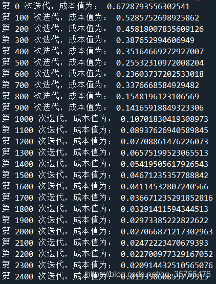
if print_cost:
print("第", i ,"次迭代,成本值为:" ,np.squeeze(cost))
#迭代完成,根据条件绘制图
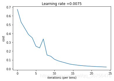
if isPlot:
plt.plot(np.squeeze(costs))
plt.ylabel('cost')
plt.xlabel('iterations (per tens)')
plt.title("Learning rate =" + str(learning_rate))
plt.show()
#返回parameters
return parameters
def predict(X, y, parameters):
"""
该函数用于预测L层神经网络的结果,当然也包含两层
参数:
X - 测试集
y - 标签
parameters - 训练模型的参数
返回:
p - 给定数据集X的预测
"""
m = X.shape[1]
n = len(parameters) // 2 # 神经网络的层数
p = np.zeros((1,m))
#根据参数前向传播
probas, caches = L_model_forward(X, parameters)
for i in range(0, probas.shape[1]):
if probas[0,i] > 0.5:
p[0,i] = 1
else:
p[0,i] = 0
print("准确度为: " + str(float(np.sum((p == y))/m)))
return p
if __name__=="__main__":
train_set_x_orig , train_set_y , test_set_x_orig , test_set_y , classes = lr_utils.load_dataset()
# train_set_x_orig.shape ; out: (209,64,64,3)
# classes out: array([b'non-cat', b'cat'], dtype='|S7')
train_x_flatten = train_set_x_orig.reshape(train_set_x_orig.shape[0], -1).T # 行数为样本数,列数为特征数,再转置得到(特征数,样本数)
test_x_flatten = test_set_x_orig.reshape(test_set_x_orig.shape[0], -1).T
train_x = train_x_flatten / 255 # 训练特征标准化
train_y = train_set_y
test_x = test_x_flatten / 255
test_y = test_set_y
n_x = 12288 # 一张图片含有的特征数,64*64*3=12288 即输入层节点数
n_h = 7 # 隐藏层节点数
n_y = 1 # 一张图片经过神经网络计算后输出y的个数 即输出层节点数
layers_dims = (n_x,n_h,n_y)
# 对参数进行更新
parameters = two_layer_model(train_x, train_set_y, layers_dims = (n_x, n_h, n_y), num_iterations = 2500, print_cost=True,isPlot=True)
predictions_train = predict(train_x, train_y, parameters) #训练集
predictions_test = predict(test_x, test_y, parameters) #测试集
结果:
- numpy.asarray()
- numpy.where() 用法详解
np.where会输出每个满足条件元素的对应坐标,原数组是几维,就输出几个数组。
多层神经网络的实现和本地图片测试
import numpy as np
import h5py
import matplotlib.pyplot as plt
import testCases #参见资料包,或者在文章底部copy
from dnn_utils import sigmoid, sigmoid_backward, relu, relu_backward #参见资料包
import lr_utils #参见资料包,或者在文章底部copy

np.random.seed(1)
def initialize_parameters_deep(layers_dims):
    """
    此函数是为了初始化多层网络参数而使用的函数。
    参数:
        layers_dims - 包含我们网络中每个图层的节点数量的列表

    返回:
        parameters - 包含参数“W1”,“b1”,...,“WL”,“bL”的字典:
                     W1 - 权重矩阵,维度为(layers_dims [1],layers_dims [1-1])
                     bl - 偏向量,维度为(layers_dims [1],1)
    """
    np.random.seed(3)
    parameters = {}
    L = len(layers_dims)

    for l in range(1,L):
        # parameters["W" + str(l)] = np.random.randn(layers_dims[l], layers_dims[l - 1]) * 0.01
        parameters["W" + str(l)] = np.random.randn(layers_dims[l], layers_dims[l - 1]) / np.sqrt(layers_dims[l - 1])
        # 使用*0.01导致了梯度消失

        parameters["b" + str(l)] = np.zeros((layers_dims[l], 1))

        #确保我要的数据的格式是正确的
        assert(parameters["W" + str(l)].shape == (layers_dims[l], layers_dims[l-1]))
        assert(parameters["b" + str(l)].shape == (layers_dims[l], 1))

    return parameters

def linear_forward(A,W,b):
    """
    实现前向传播的线性部分。

    参数:
        A - 来自上一层(或输入数据)的激活,维度为(上一层的节点数量,示例的数量)
        W - 权重矩阵,numpy数组,维度为(当前图层的节点数量,前一图层的节点数量)
        b - 偏向量,numpy向量,维度为(当前图层节点数量,1)

    返回:
         Z - 激活功能的输入,也称为预激活参数
         cache - 一个包含“A”,“W”和“b”的字典,存储这些变量以有效地计算后向传递
    """
    Z = np.dot(W,A) + b
    assert(Z.shape == (W.shape[0],A.shape[1]))
    cache = (A,W,b)

    return Z,cache

def linear_activation_forward(A_prev,W,b,activation):
    """
    实现LINEAR-> ACTIVATION 这一层的前向传播

    参数:
        A_prev - 来自上一层(或输入层)的激活,维度为(上一层的节点数量,示例数)
        W - 权重矩阵,numpy数组,维度为(当前层的节点数量,前一层的大小)
        b - 偏向量,numpy阵列,维度为(当前层的节点数量,1)
        activation - 选择在此层中使用的激活函数名,字符串类型,【"sigmoid" | "relu"】

    返回:
        A - 激活函数的输出,也称为激活后的值
        cache - 一个包含“linear_cache”和“activation_cache”的字典,我们需要存储它以有效地计算后向传递
    """

    if activation == "sigmoid":
        Z, linear_cache = linear_forward(A_prev, W, b)
        A, activation_cache = sigmoid(Z)
    elif activation == "relu":
        Z, linear_cache = linear_forward(A_prev, W, b)
        A, activation_cache = relu(Z)

    assert(A.shape == (W.shape[0],A_prev.shape[1]))
    cache = (linear_cache,activation_cache)

    return A,cache

# #测试linear_forward
# print("==============测试linear_forward==============")
# A,W,b = testCases.linear_forward_test_case()
# Z,linear_cache = linear_forward(A,W,b)
# print("Z = " + str(Z))

def L_model_forward(X,parameters):
    """
    实现[LINEAR-> RELU] *(L-1) - > LINEAR-> SIGMOID计算前向传播,也就是多层网络的前向传播,为后面每一层都执行LINEAR和ACTIVATION

    参数:
        X - 数据,numpy数组,维度为(输入节点数量,示例数)
        parameters - initialize_parameters_deep()的输出

    返回:
        AL - 最后的激活值
        caches - 包含以下内容的缓存列表:
                 linear_relu_forward()的每个cache(有L-1个,索引为从0到L-2)
                 linear_sigmoid_forward()的cache(只有一个,索引为L-1)
    """
    caches = []
    A = X
    L = len(parameters) // 2
    for l in range(1,L):
        A_prev = A
        A, cache = linear_activation_forward(A_prev, parameters['W' + str(l)], parameters['b' + str(l)], "relu")
        caches.append(cache)

    AL, cache = linear_activation_forward(A, parameters['W' + str(L)], parameters['b' + str(L)], "sigmoid")
    caches.append(cache)

    assert(AL.shape == (1,X.shape[1]))

    return AL,caches

# #测试L_model_forward
# print("==============测试L_model_forward==============")
# X,parameters = testCases.L_model_forward_test_case()
# AL,caches = L_model_forward(X,parameters)
# print("AL = " + str(AL))
# print("caches 的长度为 = " + str(len(caches)))

def compute_cost(AL,Y):
    """
    实施等式(4)定义的成本函数。

    参数:
        AL - 与标签预测相对应的概率向量,维度为(1,示例数量)
        Y - 标签向量(例如:如果不是猫,则为0,如果是猫则为1),维度为(1,数量)

    返回:
        cost - 交叉熵成本
    """
    m = Y.shape[1]
    cost = -np.sum(np.multiply(np.log(AL),Y) + np.multiply(np.log(1 - AL), 1 - Y)) / m
    # type(cost) out:<class 'numpy.float64'>
    cost = np.squeeze(cost) #从数组的形状中删除单维条目,即把shape中为1的维度去掉
    assert(cost.shape == ())

    return cost
# #测试compute_cost
# print("==============测试compute_cost==============")
# Y,AL = testCases.compute_cost_test_case()
# print("cost = " + str(compute_cost(AL, Y)))

def linear_backward(dZ,cache):
    """
    为单层实现反向传播的线性部分(第L层)

    参数:
         dZ - 相对于(当前第l层的)线性输出的成本梯度
         cache - 来自当前层前向传播的值的元组(A_prev,W,b)

    返回:
         dA_prev - 相对于激活(前一层l-1)的成本梯度,与A_prev维度相同
         dW - 相对于W(当前层l)的成本梯度,与W的维度相同
         db - 相对于b(当前层l)的成本梯度,与b维度相同
    """
    A_prev, W, b = cache
    m = A_prev.shape[1]
    dW = np.dot(dZ, A_prev.T) / m
    db = np.sum(dZ, axis=1, keepdims=True) / m
    dA_prev = np.dot(W.T, dZ)

    assert (dA_prev.shape == A_prev.shape)
    assert (dW.shape == W.shape)
    assert (db.shape == b.shape)

    return dA_prev, dW, db

# #测试linear_backward
# print("==============测试linear_backward==============")
# dZ, linear_cache = testCases.linear_backward_test_case()

# dA_prev, dW, db = linear_backward(dZ, linear_cache)
# print ("dA_prev = "+ str(dA_prev))
# print ("dW = " + str(dW))
# print ("db = " + str(db))

def linear_activation_backward(dA,cache,activation="relu"): # activation默认relu
    """
    实现LINEAR-> ACTIVATION层的后向传播。

    参数:
         dA - 当前层l的激活后的梯度值
         cache - 我们存储的用于有效计算反向传播的值的元组(值为linear_cache,activation_cache)
         activation - 要在此层中使用的激活函数名,字符串类型,【"sigmoid" | "relu"】
    返回:
         dA_prev - 相对于激活(前一层l-1)的成本梯度值,与A_prev维度相同
         dW - 相对于W(当前层l)的成本梯度值,与W的维度相同
         db - 相对于b(当前层l)的成本梯度值,与b的维度相同
    """
    linear_cache, activation_cache = cache
    if activation == "relu":
        dZ = relu_backward(dA, activation_cache)
        dA_prev, dW, db = linear_backward(dZ, linear_cache)
    elif activation == "sigmoid":
        dZ = sigmoid_backward(dA, activation_cache)
        dA_prev, dW, db = linear_backward(dZ, linear_cache)

    return dA_prev,dW,db

# #测试linear_activation_backward
# print("==============测试linear_activation_backward==============")
# AL, linear_activation_cache = testCases.linear_activation_backward_test_case()

# dA_prev, dW, db = linear_activation_backward(AL, linear_activation_cache, activation = "sigmoid")
# print ("sigmoid:")
# print ("dA_prev = "+ str(dA_prev))
# print ("dW = " + str(dW))
# print ("db = " + str(db) + "\n")

# dA_prev, dW, db = linear_activation_backward(AL, linear_activation_cache, activation = "relu")
# print ("relu:")
# print ("dA_prev = "+ str(dA_prev))
# print ("dW = " + str(dW))
# print ("db = " + str(db))

def L_model_backward(AL,Y,caches):
    """
    对[LINEAR-> RELU] *(L-1) - > LINEAR - > SIGMOID组执行反向传播,就是多层网络的向后传播

    参数:
     AL - 概率向量,正向传播的输出(L_model_forward())
     Y - 标签向量(例如:如果不是猫,则为0,如果是猫则为1),维度为(1,数量)
     caches - 包含以下内容的cache列表:
                 linear_activation_forward("relu")的cache,不包含输出层
                 linear_activation_forward("sigmoid")的cache

    返回:
     grads - 具有梯度值的字典
              grads [“dA”+ str(l)] = ...
              grads [“dW”+ str(l)] = ...
              grads [“db”+ str(l)] = ...
    """
    grads = {}
    L = len(caches)
    m = AL.shape[1]
    Y = Y.reshape(AL.shape)     # 使a和y纬度相同
    dAL = - (np.divide(Y, AL) - np.divide(1 - Y, 1 - AL))

    current_cache = caches[L-1] # cache从0开始L-1存放的是第L层的正向缓存
    grads["dA" + str(L)], grads["dW" + str(L)], grads["db" + str(L)] = linear_activation_backward(dAL, current_cache, "sigmoid")

    for l in reversed(range(L-1)):  # 从l=L-2开始 到l=0
        current_cache = caches[l]
        dA_prev_temp, dW_temp, db_temp = linear_activation_backward(grads["dA" + str(l + 2)], current_cache, "relu")
        # 计算L-1层的dA,dW,db,需要用到第L层的数据,所以第一次循环传入dAL和current_cache[L-2](current_cache[L-2]实际存放的是L-1层的正向缓存)
        grads["dA" + str(l + 1)] = dA_prev_temp
        grads["dW" + str(l + 1)] = dW_temp
        grads["db" + str(l + 1)] = db_temp

    return grads

# #测试L_model_backward
# print("==============测试L_model_backward==============")
# AL, Y_assess, caches = testCases.L_model_backward_test_case()
# grads = L_model_backward(AL, Y_assess, caches)
# print ("dW1 = "+ str(grads["dW1"]))
# print ("db1 = "+ str(grads["db1"]))
# print ("dA1 = "+ str(grads["dA1"]))

def update_parameters(parameters, grads, learning_rate):
    """
    使用梯度下降更新参数

    参数:
     parameters - 包含你的参数的字典
     grads - 包含梯度值的字典,是L_model_backward的输出

    返回:
     parameters - 包含更新参数的字典
                   参数[“W”+ str(l)] = ...
                   参数[“b”+ str(l)] = ...
    """
    L = len(parameters) // 2 #整除
    for l in range(L):
        parameters["W" + str(l + 1)] = parameters["W" + str(l + 1)] - learning_rate * grads["dW" + str(l + 1)]
        parameters["b" + str(l + 1)] = parameters["b" + str(l + 1)] - learning_rate * grads["db" + str(l + 1)]

    return parameters

# #测试update_parameters
# print("==============测试update_parameters==============")
# parameters, grads = testCases.update_parameters_test_case()
# parameters = update_parameters(parameters, grads, 0.1)

# print ("W1 = "+ str(parameters["W1"]))
# print ("b1 = "+ str(parameters["b1"]))
# print ("W2 = "+ str(parameters["W2"]))
# print ("b2 = "+ str(parameters["b2"]))

def two_layer_model(X,Y,layers_dims,learning_rate=0.0075,num_iterations=3000,print_cost=False,isPlot=True):
    """
    实现一个两层的神经网络,【LINEAR->RELU】 -> 【LINEAR->SIGMOID】
    参数:
        X - 输入的数据,维度为(n_x,例子数)
        Y - 标签,向量,0为非猫,1为猫,维度为(1,数量)
        layers_dims - 层数的向量,维度为(n_y,n_h,n_y)
        learning_rate - 学习率
        num_iterations - 迭代的次数
        print_cost - 是否打印成本值,每100次打印一次
        isPlot - 是否绘制出误差值的图谱
    返回:
        parameters - 一个包含W1,b1,W2,b2的字典变量
    """
    np.random.seed(1)
    grads = {}
    costs = []
    (n_x,n_h,n_y) = layers_dims

    """
    初始化参数
    """
    parameters = initialize_parameters_deep(layers_dims)

    W1 = parameters["W1"]
    b1 = parameters["b1"]
    W2 = parameters["W2"]
    b2 = parameters["b2"]

    """
    开始进行迭代
    """
    for i in range(0,num_iterations):
        #前向传播
        A1, cache1 = linear_activation_forward(X, W1, b1, "relu")
        A2, cache2 = linear_activation_forward(A1, W2, b2, "sigmoid")

        #计算成本
        cost = compute_cost(A2,Y)

        #后向传播
        ##初始化后向传播
        dA2 = - (np.divide(Y, A2) - np.divide(1 - Y, 1 - A2))

        ##向后传播,输入:“dA2,cache2,cache1”。 输出:“dA1,dW2,db2;还有dA0(未使用),dW1,db1”。
        dA1, dW2, db2 = linear_activation_backward(dA2, cache2, "sigmoid")
        dA0, dW1, db1 = linear_activation_backward(dA1, cache1, "relu")

        ##向后传播完成后的数据保存到grads
        grads["dW1"] = dW1
        grads["db1"] = db1
        grads["dW2"] = dW2
        grads["db2"] = db2

        #更新参数
        parameters = update_parameters(parameters,grads,learning_rate)
        W1 = parameters["W1"]
        b1 = parameters["b1"]
        W2 = parameters["W2"]
        b2 = parameters["b2"]

        #打印成本值,如果print_cost=False则忽略
        if i % 100 == 0:
            #记录成本
            costs.append(cost)
            #是否打印成本值
            if print_cost:
                print("第", i ,"次迭代,成本值为:" ,np.squeeze(cost))
    #迭代完成,根据条件绘制图
    if isPlot:
        plt.plot(np.squeeze(costs))
        plt.ylabel('cost')
        plt.xlabel('iterations (per tens)')
        plt.title("Learning rate =" + str(learning_rate))
        plt.show()

    #返回parameters
    return parameters

def L_layer_model(X, Y, layers_dims, learning_rate=0.0075, num_iterations=3000, print_cost=False,isPlot=True):
    """
    实现一个L层神经网络:[LINEAR-> RELU] *(L-1) - > LINEAR-> SIGMOID。

    参数:
	    X - 输入的数据,维度为(n_x,例子数)
        Y - 标签,向量,0为非猫,1为猫,维度为(1,数量)
        layers_dims - 层数的向量,维度为(n_y,n_h,···,n_h,n_y)
        learning_rate - 学习率
        num_iterations - 迭代的次数
        print_cost - 是否打印成本值,每100次打印一次
        isPlot - 是否绘制出误差值的图谱

    返回:
     parameters - 模型学习的参数。 然后他们可以用来预测。
    """
    np.random.seed(1)
    costs = []

    parameters = initialize_parameters_deep(layers_dims)

    for i in range(0,num_iterations):
        AL , caches = L_model_forward(X,parameters)
        cost = compute_cost(AL,Y)
        grads = L_model_backward(AL,Y,caches)
        parameters = update_parameters(parameters,grads,learning_rate)

        #打印成本值,如果print_cost=False则忽略
        if i % 100 == 0:
            #记录成本
            costs.append(cost)
            #是否打印成本值
            if print_cost:
                print("第", i ,"次迭代,成本值为:" ,np.squeeze(cost))
    #迭代完成,根据条件绘制图
    if isPlot:
        plt.plot(np.squeeze(costs))
        plt.ylabel('cost')
        plt.xlabel('iterations (per tens)')
        plt.title("Learning rate =" + str(learning_rate))
        plt.show()
    return parameters

def print_mislabeled_images(classes, X, y, p):
    """
	绘制预测和实际不同的图像。
	    X - 数据集
	    y - 实际的标签
	    p - 预测
    """
    a = p + y
    mislabeled_indices = np.asarray(np.where(a == 1))   # 返回位置索引
    plt.rcParams['figure.figsize'] = (40.0, 40.0) # set default size of plots
    num_images = len(mislabeled_indices[0])
    for i in range(num_images):
        index = mislabeled_indices[1][i]    # 因为a导致mislabeled_indices为二维,所以要先索引[1]

        plt.subplot(2, num_images, i + 1)
        plt.imshow(X[:,index].reshape(64,64,3), interpolation='nearest')
        plt.axis('off')
        plt.title("Prediction: " + classes[int(p[0,index])].decode("utf-8") + " \n Class: " + classes[y[0,index]].decode("utf-8"))


def predict(X, y, parameters):
    """
    该函数用于预测L层神经网络的结果,当然也包含两层

    参数:
     X - 测试集
     y - 标签
     parameters - 训练模型的参数

    返回:
     p - 给定数据集X的预测
    """

    m = X.shape[1]
    n = len(parameters) // 2 # 神经网络的层数
    p = np.zeros((1,m))

    #根据参数前向传播
    probas, caches = L_model_forward(X, parameters)

    for i in range(0, probas.shape[1]):
        if probas[0,i] > 0.5:
            p[0,i] = 1
        else:
            p[0,i] = 0

    print("准确度为: "  + str(float(np.sum((p == y))/m)))

    return p


if __name__=="__main__":
    train_set_x_orig , train_set_y , test_set_x_orig , test_set_y , classes = lr_utils.load_dataset()
    # train_set_x_orig.shape ; out: (209,64,64,3)
    # classes out: array([b'non-cat', b'cat'], dtype='|S7')
    train_x_flatten = train_set_x_orig.reshape(train_set_x_orig.shape[0], -1).T     # 行数为样本数,列数为特征数,再转置得到(特征数,样本数)
    test_x_flatten = test_set_x_orig.reshape(test_set_x_orig.shape[0], -1).T

    train_x = train_x_flatten / 255  # 训练特征标准化
    train_y = train_set_y
    test_x = test_x_flatten / 255
    test_y = test_set_y

    # 两层神经网络
    # n_x = 12288     # 一张图片含有的特征数,64*64*3=12288 即输入层节点数
    # n_h = 7         # 隐藏层节点数
    # n_y = 1         # 一张图片经过神经网络计算后输出y的个数 即输出层节点数
    # layers_dims = (n_x,n_h,n_y)
    # # 对参数进行更新
    # parameters = two_layer_model(train_x, train_set_y, layers_dims = (n_x, n_h, n_y), num_iterations = 2500, print_cost=True,isPlot=True)
    # predictions_train = predict(train_x, train_y, parameters) #训练集
    # predictions_test = predict(test_x, test_y, parameters) #测试集

    # 多层神经网络
    layers_dims = [12288, 20, 7, 5, 1] #  5-layer model

    parameters = L_layer_model(train_x, train_y, layers_dims, num_iterations = 2500, print_cost = True,isPlot=True)
    pred_train = predict(train_x, train_y, parameters) #训练集
    pred_test = predict(test_x, test_y, parameters) #测试集

    # 输出被错判断的图片
    print_mislabeled_images(classes, test_x, test_y, pred_test)


    ## START CODE HERE ##
    # 使用自己本地的图片测试
    from PIL import Image
    my_image = "cat.jpg" # change this to the name of your image file
    my_label_y = [1]
    num_px = 64
    fname =  "images/" + my_image
    # 读取图片,将其转化为三通道,并resize为64*64分辨率
    image = Image.open(fname).convert("RGB").resize((num_px, num_px))
    # 将图片转化为矩阵形式并reshape以满足模型输入格式
    my_image = np.array(image).reshape(num_px*num_px * 3, -1)
    my_predict_image = predict(my_image,my_label_y,parameters)
    plt.imshow(image)


 1358
1358

 被折叠的 条评论
为什么被折叠?
被折叠的 条评论
为什么被折叠?
 到【灌水乐园】发言


