seaborn可视化

import matplotlib.pyplot as plt
%matplotlib inline
import seaborn as sns
sns.set()
import numpy as np
import pandas as pd

In [8]:

data=np.random.multivariate_normal([0,0],[[5,2],[2,2]],size=2000)

data=pd.DataFrame(data,columns=['x','y'])

In [9]:

data.head()

Out[9]:

	x	y
0	0.571117	-0.158731
1	2.522765	2.033863
2	-3.413121	-0.566827
3	-1.788482	-0.308131
4	3.565947	2.668333

In [10]:

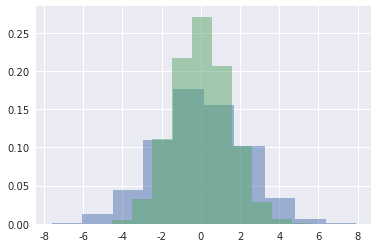
for col in 'xy':#频次直方图
    plt.hist(data[col],normed=True,alpha=0.5)

/opt/conda/lib/python3.5/site-packages/matplotlib/axes/_axes.py:6462: UserWarning: The 'normed' kwarg is deprecated, and has been replaced by the 'density' kwarg.
  warnings.warn("The 'normed' kwarg is deprecated, and has been "

In [11]:

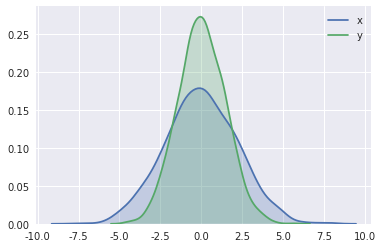
for col in 'xy':#KDE可视化
    sns.kdeplot(data[col],shade=True)

In [14]:

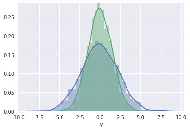
sns.distplot(data['x'])#频次直方图与KDE的结合
sns.distplot(data['y']);

/opt/conda/lib/python3.5/site-packages/matplotlib/axes/_axes.py:6462: UserWarning: The 'normed' kwarg is deprecated, and has been replaced by the 'density' kwarg.
  warnings.warn("The 'normed' kwarg is deprecated, and has been "

In [15]:

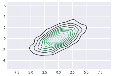
sns.kdeplot(data);#二维KDE图

/opt/conda/lib/python3.5/site-packages/seaborn/distributions.py:645: UserWarning: Passing a 2D dataset for a bivariate plot is deprecated in favor of kdeplot(x, y), and it will cause an error in future versions. Please update your code.
  warnings.warn(warn_msg, UserWarning)

In [18]:

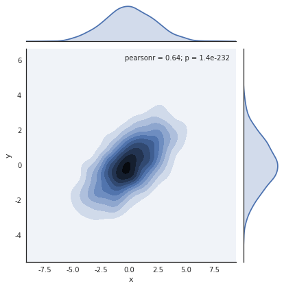
with sns.axes_style('white'):
    sns.jointplot('x','y',data,kind='kde')

In [19]:

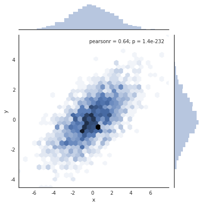
with sns.axes_style('white'):
    sns.jointplot('x','y',data,kind='hex')

/opt/conda/lib/python3.5/site-packages/matplotlib/axes/_axes.py:6462: UserWarning: The 'normed' kwarg is deprecated, and has been replaced by the 'density' kwarg.
  warnings.warn("The 'normed' kwarg is deprecated, and has been "

In [20]:

iris=sns.load_dataset('iris')

In [21]:

iris.head()

Out[21]:

	sepal_length	sepal_width	petal_length	petal_width	species
0	5.1	3.5	1.4	0.2	setosa
1	4.9	3.0	1.4	0.2	setosa
2	4.7	3.2	1.3	0.2	setosa
3	4.6	3.1	1.5	0.2	setosa
4	5.0	3.6	1.4	0.2	setosa

In [24]:

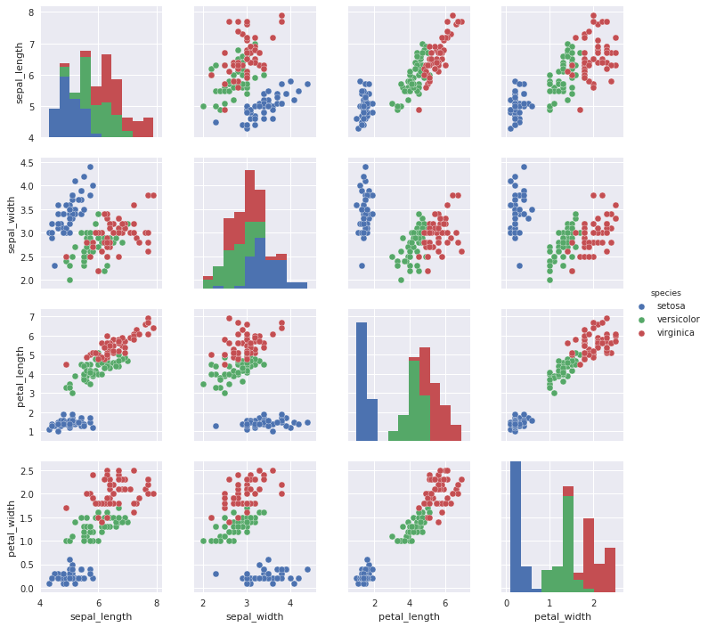
sns.pairplot(iris,hue='species',size=2.5)#矩阵图

Out[24]:

<seaborn.axisgrid.PairGrid at 0x7f380c3ac0b8>

In [26]:

tips=sns.load_dataset('tips')
tips.head()

Out[26]:

	total_bill	tip	sex	smoker	day	time	size
0	16.99	1.01	Female	No	Sun	Dinner	2
1	10.34	1.66	Male	No	Sun	Dinner	3
2	21.01	3.50	Male	No	Sun	Dinner	3
3	23.68	3.31	Male	No	Sun	Dinner	2
4	24.59	3.61	Female	No	Sun	Dinner	4

In [32]:

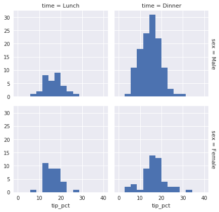
tips['tip_pct']=100*tips['tip']/tips['total_bill']#分面频次直方图
grid=sns.FacetGrid(tips,row='sex',col='time',margin_titles=True)
grid.map(plt.hist,'tip_pct',bins=np.linspace(0,40,15));

In [35]:

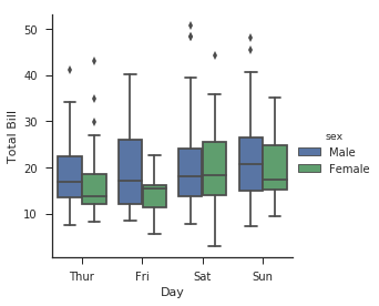
with sns.axes_style(style='ticks'):  # 因子图中不同离散因子分布对比
    g = sns.factorplot('day', 'total_bill', 'sex', data=tips, kind='box')
    g.set_axis_labels('Day', 'Total Bill')

In [37]:

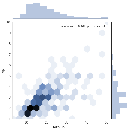
with sns.axes_style('white'):#联合分布图
    sns.jointplot('total_bill','tip',data=tips,kind='hex')

/opt/conda/lib/python3.5/site-packages/matplotlib/axes/_axes.py:6462: UserWarning: The 'normed' kwarg is deprecated, and has been replaced by the 'density' kwarg.
  warnings.warn("The 'normed' kwarg is deprecated, and has been "

In [38]:

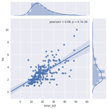
sns.jointplot('total_bill','tip',data=tips,kind='reg')#带回归拟合的联合分布

/opt/conda/lib/python3.5/site-packages/matplotlib/axes/_axes.py:6462: UserWarning: The 'normed' kwarg is deprecated, and has been replaced by the 'density' kwarg.
  warnings.warn("The 'normed' kwarg is deprecated, and has been "

Out[38]:

<seaborn.axisgrid.JointGrid at 0x7f37faf14dd8>

In [40]:

planets=sns.load_dataset('planets')#用行星数据
planets.head()

Out[40]:

	method	number	orbital_period	mass	distance	year
0	Radial Velocity	1	269.300	7.10	77.40	2006
1	Radial Velocity	1	874.774	2.21	56.95	2008
2	Radial Velocity	1	763.000	2.60	19.84	2011
3	Radial Velocity	1	326.030	19.40	110.62	2007
4	Radial Velocity	1	516.220	10.50	119.47	2009

In [41]:

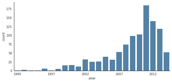
with sns.axes_style('white'):
    g=sns.factorplot('year',data=planets,aspect=2,kind='count',color='steelblue')
    g.set_xticklabels(step=5)

In [42]:

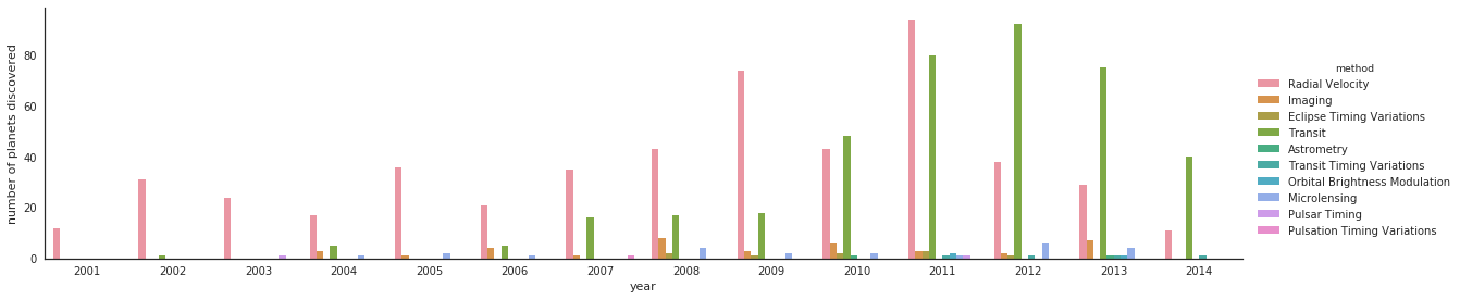
with sns.axes_style('white'):#不同年份、方法发现的行星数量
    g=sns.factorplot('year',data=planets,aspect=4.0,kind='count',hue='method',order=range(2001,2015))
    g.set_ylabels('number of planets discovered')