【ML】线性回归 の 不受异常值影响的线性回归方案

---

问题发现

因为高频的数据波动性很大，经常出现坏点，于是思考如何对这样的坏点做linear regression而不用担心ols estimation太过sensitive的难题。

解决方案

Solution1：R/python Least Absolute Deviation(LAD)

即最小化与模型diff的绝对值而不是squares。

• R 有 rqPen 和 hqreg 这两个包可以做quantile regression，下面可二选一：

  • median regression
  • 50% percentile的quantile regression

• python 只有这个小包，内部实现用 tensorflow：https://mirca.github.io/lad/

Solution2：python statsmodels RLM

• 算法：Estimate a robust linear model via iteratively reweighted least squares given a robust criterion estimator. 在给定稳健标准估计量的情况下，通过迭代重新加权最小二乘法估计稳健线性模型。
• 🔗：https://www.statsmodels.org/dev/generated/statsmodels.robust.robust_linear_model.RLM.html

Solution3：python sklearn RANSAC

• 算法：In this example we see how to robustly fit a linear model to faulty data using the RANSAC algorithm. 在本例中，我们将看到如何使用 RANSAC 算法将线性模型稳健地拟合到错误数据中。这个包用了scipy的RANSAC算法包。这个算法也用了“内点””外点“的模型，准倒是准，需要迭代所以运算速度比较慢。
• 🔗：https://scikit-learn.org/stable/auto_examples/linear_model/plot_ransac.html

---

简例

# Robustly fit linear model with RANSAC algorithm
ransac = linear_model.RANSACRegressor()
ransac.fit(X, y)

Estimated coefficients (true, linear regression, RANSAC):
82.1903908407869 [54.17236387] [82.08533159]

---

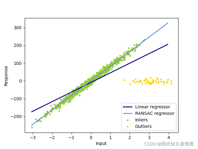
完整code

import numpy as np
from matplotlib import pyplot as plt

from sklearn import linear_model, datasets


n_samples = 1000
n_outliers = 50


X, y, coef = datasets.make_regression(
    n_samples=n_samples,
    n_features=1,
    n_informative=1,
    noise=10,
    coef=True,
    random_state=0,
)

# Add outlier data
np.random.seed(0)
X[:n_outliers] = 3 + 0.5 * np.random.normal(size=(n_outliers, 1))
y[:n_outliers] = -3 + 10 * np.random.normal(size=n_outliers)

# Fit line using all data
lr = linear_model.LinearRegression()
lr.fit(X, y)

# Robustly fit linear model with RANSAC algorithm
ransac = linear_model.RANSACRegressor()
ransac.fit(X, y)
inlier_mask = ransac.inlier_mask_
outlier_mask = np.logical_not(inlier_mask)

# Predict data of estimated models
line_X = np.arange(X.min(), X.max())[:, np.newaxis]
line_y = lr.predict(line_X)
line_y_ransac = ransac.predict(line_X)

# Compare estimated coefficients
print("Estimated coefficients (true, linear regression, RANSAC):")
print(coef, lr.coef_, ransac.estimator_.coef_)

lw = 2
plt.scatter(
    X[inlier_mask], y[inlier_mask], color="yellowgreen", marker=".", label="Inliers"
)
plt.scatter(
    X[outlier_mask], y[outlier_mask], color="gold", marker=".", label="Outliers"
)
plt.plot(line_X, line_y, color="navy", linewidth=lw, label="Linear regressor")
plt.plot(
    line_X,
    line_y_ransac,
    color="cornflowerblue",
    linewidth=lw,
    label="RANSAC regressor",
)
plt.legend(loc="lower right")
plt.xlabel("Input")
plt.ylabel("Response")
plt.show()

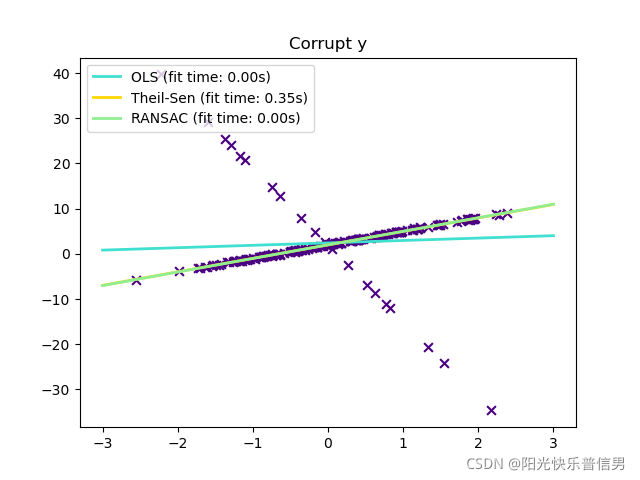
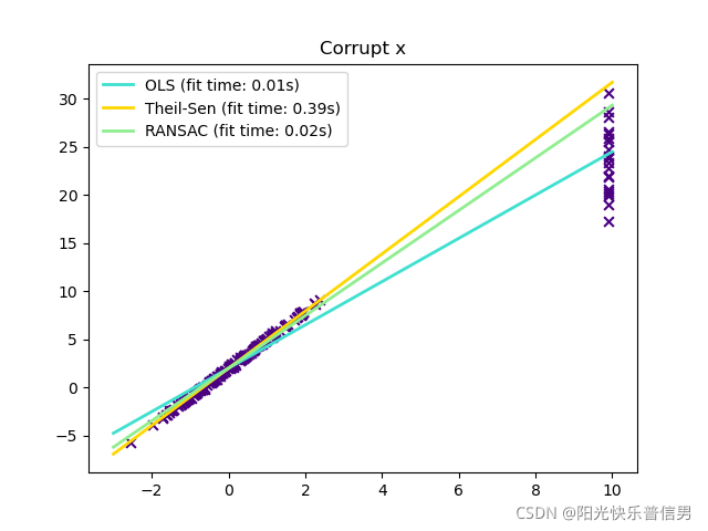
Solution4：python sklearn Theil-Sen

• 算法：也是分组算法，和RANSAC类似。generalized-median-based estimator，算法中使用median实现稳定性。比RANSAC还慢。

• 🔗：https://scikit-learn.org/stable/auto_examples/linear_model/plot_ransac.html

---

完整code

# Author: Florian Wilhelm -- <florian.wilhelm@gmail.com>
# License: BSD 3 clause

import time
import numpy as np
import matplotlib.pyplot as plt
from sklearn.linear_model import LinearRegression, TheilSenRegressor
from sklearn.linear_model import RANSACRegressor

estimators = [
    ("OLS", LinearRegression()),
    ("Theil-Sen", TheilSenRegressor(random_state=42)),
    ("RANSAC", RANSACRegressor(random_state=42)),
]
colors = {"OLS": "turquoise", "Theil-Sen": "gold", "RANSAC": "lightgreen"}
lw = 2

# #############################################################################
# Outliers only in the y direction

np.random.seed(0)
n_samples = 200
# Linear model y = 3*x + N(2, 0.1**2)
x = np.random.randn(n_samples)
w = 3.0
c = 2.0
noise = 0.1 * np.random.randn(n_samples)
y = w * x + c + noise
# 10% outliers
y[-20:] += -20 * x[-20:]
X = x[:, np.newaxis]

plt.scatter(x, y, color="indigo", marker="x", s=40)
line_x = np.array([-3, 3])
for name, estimator in estimators:
    t0 = time.time()
    estimator.fit(X, y)
    elapsed_time = time.time() - t0
    y_pred = estimator.predict(line_x.reshape(2, 1))
    plt.plot(
        line_x,
        y_pred,
        color=colors[name],
        linewidth=lw,
        label="%s (fit time: %.2fs)" % (name, elapsed_time),
    )

plt.axis("tight")
plt.legend(loc="upper left")
plt.title("Corrupt y")

# #############################################################################
# Outliers in the X direction

np.random.seed(0)
# Linear model y = 3*x + N(2, 0.1**2)
x = np.random.randn(n_samples)
noise = 0.1 * np.random.randn(n_samples)
y = 3 * x + 2 + noise
# 10% outliers
x[-20:] = 9.9
y[-20:] += 22
X = x[:, np.newaxis]

plt.figure()
plt.scatter(x, y, color="indigo", marker="x", s=40)

line_x = np.array([-3, 10])
for name, estimator in estimators:
    t0 = time.time()
    estimator.fit(X, y)
    elapsed_time = time.time() - t0
    y_pred = estimator.predict(line_x.reshape(2, 1))
    plt.plot(
        line_x,
        y_pred,
        color=colors[name],
        linewidth=lw,
        label="%s (fit time: %.2fs)" % (name, elapsed_time),
    )

plt.axis("tight")
plt.legend(loc="upper left")
plt.title("Corrupt x")
plt.show()

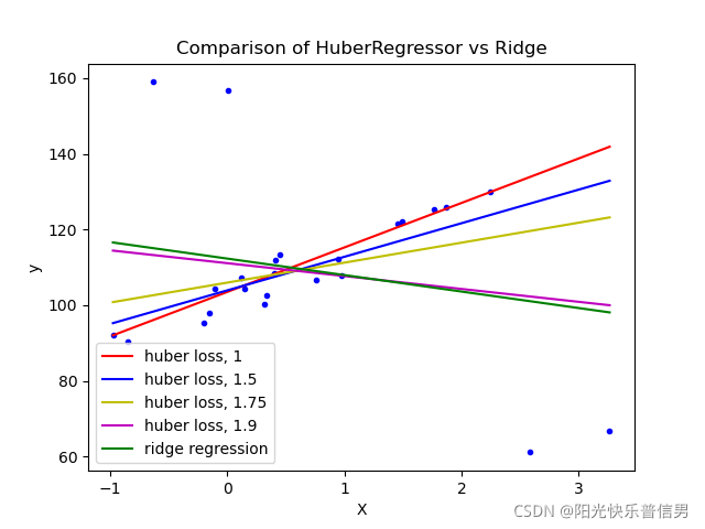
Solution5：python sklearn Huber Regression

• 算法：与ridge regression有类似的正则化效果，但是添加了outlier识别。
• 🔗：https://scikit-learn.org/stable/modules/linear_model.html#robustness-regression-outliers-and-modeling-errors