机器学习之逻辑回归(Logistic Regression)

最新推荐文章于 2025-05-18 16:55:21 发布

原创最新推荐文章于 2025-05-18 16:55:21 发布 · 1k 阅读

11 ·

CC 4.0 BY-SA版权

机器学习专栏收录该内容

20 篇文章

订阅专栏

这篇博客详细探讨了逻辑回归的原理，包括损失函数的梯度、算法实现、决策边界的理解以及如何通过添加多项式特征改进模型。同时，文章还介绍了如何使用One-vs-Rest (OVR) 和 One-vs-One (OVO)策略来解决多分类问题。

摘要生成于 C知道，由 DeepSeek-R1 满血版支持，前往体验 >

"""逻辑回归中的Sigmoid函数"""
import numpy as np
import matplotlib.pyplot as plt

def sigmoid(t):
    return 1/(1+np.exp(-t))

x=np.linspace(-10,10,500)
y=sigmoid(x)

plt.plot(x,y)
plt.show()

结果：

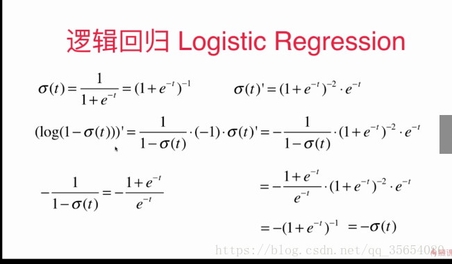
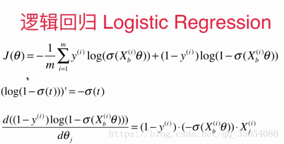
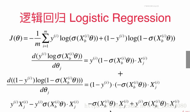
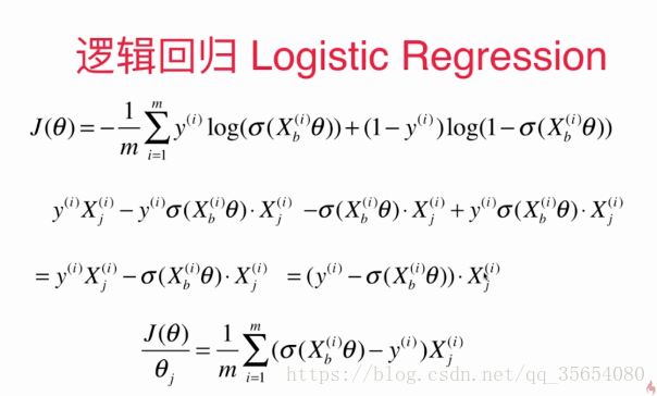
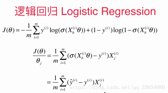
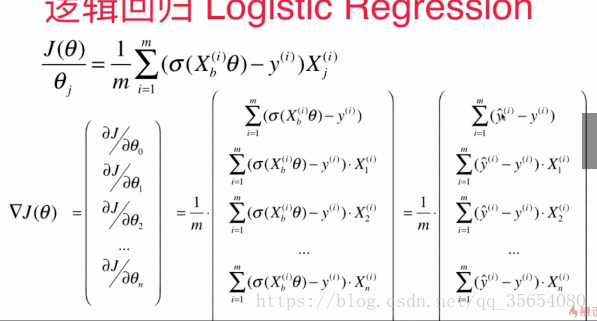
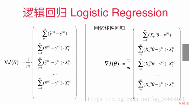
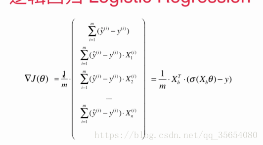
逻辑回归损失函数的梯度：

逻辑回归算法：

import numpy as np
from metrics import accuracy_score

class LogisticRegression:

    def __init__(self):
        """初始化Logistic Regression模型"""
        self.coef_ = None
        self.intercept_ = None
        self._theta = None

    def _sigmoid(self,t):
        return 1. / (1. + np.exp(-t))

    def fit(self, X_train, y_train, eta=0.01, n_iters=1e4):
        """根据训练数据集X_train, y_train, 使用梯度下降法训练Linear Regression模型"""
        assert X_train.shape[0] == y_train.shape[0], \
            "the size of X_train must be equal to the size of y_train"



        def J(theta, X_b, y):
            """求损失函数"""
            y_hat=self._sigmoid(X_b.dot(theta))
            try:
                return -np.sum(y*np.log(y_hat) + (1-y)*np.log(1-y_hat))/ len(y)
            except:
                return float('inf')

        def dJ(theta, X_b, y):
            """求梯度"""
            # res = np.empty(len(theta))
            # res[0] = np.sum(X_b.dot(theta) - y)
            # for i in range(1, len(theta)):
            #     res[i] = (X_b.dot(theta) - y).dot(X_b[:, i])
            # return res * 2 / len(X_b)
            return X_b.T.dot(self._sigmoid(X_b.dot(theta)) - y) / len(X_b)

        def gradient_descent(X_b, y, initial_theta, eta, n_iters=1e4, epsilon=1e-8):
            """使用批量梯度下降法寻找theta"""
            theta = initial_theta
            cur_iter = 0

            while cur_iter < n_iters:
                gradient = dJ(theta, X_b, y)
                last_theta = theta
                theta = theta - eta * gradient
                if (abs(J(theta, X_b, y) - J(last_theta, X_b, y)) < epsilon):
                    break

                cur_iter += 1

            return theta

        X_b = np.hstack([np.ones((len(X_train), 1)), X_train])
        initial_theta = np.zeros(X_b.shape[1])
        self._theta = gradient_descent(X_b, y_train, initial_theta, eta, n_iters)

        self.intercept_ = self._theta[0]
        self.coef_ = self._theta[1:]

        return self

    def predict_proba(self, X_predict):
        """给定待预测数据集X_predict，返回表示X_predict的结果概率向量"""
        assert self.intercept_ is not None and self.coef_ is not None, \
            "must fit before predict!"
        assert X_predict.shape[1] == len(self.coef_), \
            "the feature number of X_predict must be equal to X_train"

        X_b = np.hstack([np.ones((len(X_predict), 1)), X_predict])
        return self._sigmoid(X_b.dot(self._theta))

    def predict(self, X_predict):
        """给定待预测数据集X_predict，返回表示X_predict的结果向量"""
        assert self.intercept_ is not None and self.coef_ is not None, \
            "must fit before predict!"
        assert X_predict.shape[1] == len(self.coef_), \
            "the feature number of X_predict must be equal to X_train"

        proba=self.predict_proba(X_predict)
        return np.array(proba>=0.5,dtype='int')

    def score(self, X_test, y_test):
        """根据测试数据集 X_test 和 y_test 确定当前模型的准确度"""

        y_predict = self.predict(X_test)
        return accuracy_score(y_test, y_predict)

    def __repr__(self):
        return "LogisticRegression()"

"""实现逻辑回归"""
import numpy as np
import matplotlib.pyplot as plt
from sklearn import datasets

iris=datasets.load_iris()
X=iris.data
y=iris.target

X=X[y<2,:2]
y=y[y<2]

plt.scatter(X[y==0,0],X[y==0,1],color='red')
plt.scatter(X[y==1,0],X[y==1,1],color='blue')
plt.show()

"""使用逻辑回归"""
from model_selection import train_test_split
from LogisticRegression import LogisticRegression

X_train,X_test,y_train,y_test=train_test_split(X,y,seed=666)
log_reg=LogisticRegression()
log_reg.fit(X_train,y_train)
print(log_reg.score(X_test,y_test))
print(log_reg.predict_proba(X_test))

结果：

E:\pythonspace\KNN_function\venv\Scripts\python.exe E:/pythonspace/KNN_function/try.py
1.0
[0.92972035 0.98664939 0.14852024 0.17601199 0.0369836  0.0186637
 0.04936918 0.99669244 0.97993941 0.74524655 0.04473194 0.00339285
 0.26131273 0.0369836  0.84192923 0.79892262 0.82890209 0.32358166
 0.06535323 0.20735334]

Process finished with exit code 0

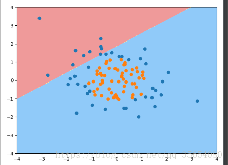
逻辑回归中的决策边界和添加多项式特征：

"""在逻辑回归中添加多项式特征"""
import numpy as np
import matplotlib.pyplot as plt

np.random.seed(666)
X=np.random.normal(0,1,size=(100,2))
y=np.array(X[:,0]**2+X[:,1]**2<1.5,dtype='int')


"""使用逻辑回归"""
from LogisticRegression import LogisticRegression

log_reg=LogisticRegression()
log_reg.fit(X,y)

"""绘制思路"""
def plot_decision_boundary(model,axis):
    x0,x1 = np.meshgrid(
        np.linspace(axis[0],axis[1],int((axis[1]-axis[0])*100)),
        np.linspace(axis[2],axis[3],int((axis[3]-axis[2])*100))
    )
    X_new = np.c_[x0.ravel(),x1.ravel()]
    y_predict = model.predict(X_new)
    zz = y_predict.reshape(x0.shape)
    from matplotlib.colors import ListedColormap
    custom_cmap = ListedColormap(['#EF9A9A','#FFF59D','#90CAF9'])
    plt.contourf(x0,x1,zz,linewidth=5,cmap=custom_cmap)

plot_decision_boundary(log_reg,axis=[-4,4,-4,4])
plt.scatter(X[y==0,0],X[y==0,1])
plt.scatter(X[y==1,0],X[y==1,1])
plt.show()


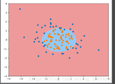
"""添加特征值，即升维"""
from sklearn.preprocessing import PolynomialFeatures
from sklearn.preprocessing import StandardScaler
from sklearn.pipeline import Pipeline
def PolynomialLogisticRegression(degree):
    return Pipeline([
        ('Poly',PolynomialFeatures(degree=degree)),
        ('std_scaler',StandardScaler()),
        ('Logistic',LogisticRegression())
    ])
poly_log_reg = PolynomialLogisticRegression(degree=2)
poly_log_reg.fit(X,y)
plot_decision_boundary(poly_log_reg,axis=[-4,4,-4,4])
plt.scatter(X[y==0,0],X[y==0,1])
plt.scatter(X[y==1,0],X[y==1,1])
plt.show()

结果：

"""逻辑回归中使用正则化"""
import numpy as np
import matplotlib.pyplot as plt
from sklearn.model_selection import train_test_split
from sklearn.linear_model import LogisticRegression
from sklearn.preprocessing import StandardScaler
from sklearn.pipeline import Pipeline
from sklearn.preprocessing import PolynomialFeatures

np.random.seed(666)
X=np.random.normal(0,1,size=(200,2))
y=np.array(X[:,0]**2+X[:,1]<1.5,dtype='int')
for _ in range(20):
    y[np.random.randint(200)] = 1
plt .scatter(X[y==0,0],X[y==0,1])
plt .scatter(X[y==1,0],X[y==1,1])
plt.show()

X_train,X_test,y_train,y_test=train_test_split(X,y)
log_reg=LogisticRegression()
log_reg.fit(X,y)
def plot_decision_boundary(model,axis):
    x0,x1 = np.meshgrid(
        np.linspace(axis[0],axis[1],int((axis[1]-axis[0])*100)),
        np.linspace(axis[2],axis[3],int((axis[3]-axis[2])*100))
    )
    X_new = np.c_[x0.ravel(),x1.ravel()]
    y_predict = model.predict(X_new)
    zz = y_predict.reshape(x0.shape)
    from matplotlib.colors import ListedColormap
    custom_cmap = ListedColormap(['#EF9A9A','#FFF59D','#90CAF9'])
    plt.contourf(x0,x1,zz,linewidth=5,cmap=custom_cmap)

def PolynomialLogisticRegression(degree,C=1.0,penalty='l2'):
    return Pipeline([
    ('Poly',PolynomialFeatures(degree=degree)),
    ('std_scaler',StandardScaler()),
    ('Logistic',LogisticRegression(C=C,penalty=penalty))
])
poly_log_reg = PolynomialLogisticRegression(degree=20,C=0.1,penalty='l1')
poly_log_reg.fit(X_train,y_train)

plot_decision_boundary(poly_log_reg,axis=[-4,4,-4,4])
plt.scatter(X[y==0,0],X[y==0,1])
plt.scatter(X[y==1,0],X[y==1,1])
plt.show()

结果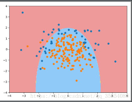

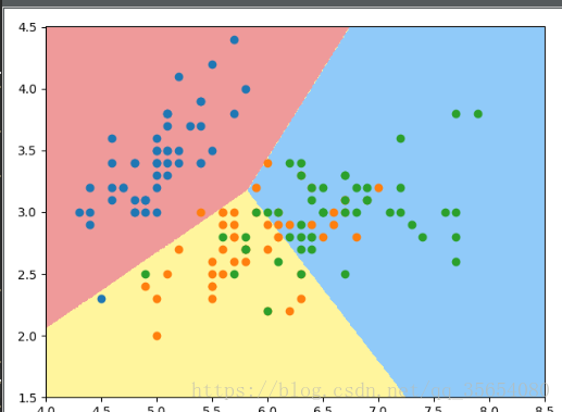
应用OVR和OVO使逻辑回归处理多分类问题

"""OVR和OVO"""
#为了数据可视化方便，我们只使用鸢尾花数据集的前两列特征
from sklearn import datasets
from sklearn.linear_model import LogisticRegression
from sklearn.model_selection import train_test_split
import matplotlib.pyplot as plt
import numpy as np

iris = datasets.load_iris()
X = iris['data'][:,:2]
y = iris['target']
X_train,X_test,y_train,y_test=train_test_split(X,y,random_state=666)


#log_reg = LogisticRegression(multi_class='ovr')   #传入multi_class参数可以指定使用ovr或ovo，默认ovr   #由于只使用前两列特征，导致分类准确度较低
log_reg = LogisticRegression(multi_class='ovr',solver='newton-cg')
log_reg.fit(X_train,y_train)
log_reg.score(X_test,y_test)
def plot_decision_boundary(model,axis):
    x0,x1 = np.meshgrid(
        np.linspace(axis[0],axis[1],int((axis[1]-axis[0])*100)),
        np.linspace(axis[2],axis[3],int((axis[3]-axis[2])*100))
    )
    X_new = np.c_[x0.ravel(),x1.ravel()]
    y_predict = model.predict(X_new)
    zz = y_predict.reshape(x0.shape)
    from matplotlib.colors import ListedColormap
    custom_cmap = ListedColormap(['#EF9A9A','#FFF59D','#90CAF9'])
    plt.contourf(x0,x1,zz,linewidth=5,cmap=custom_cmap)

plot_decision_boundary(log_reg,axis=[4,8.5,1.5,4.5])
plt.scatter(X[y==0,0],X[y==0,1])
plt.scatter(X[y==1,0],X[y==1,1])
plt.scatter(X[y==2,0],X[y==2,1])
plt.show()



"""使用全部数据 OVR and OVO"""
from sklearn.multiclass import OneVsOneClassifier
from sklearn.multiclass import OneVsRestClassifier

from sklearn import datasets
from sklearn.linear_model import LogisticRegression
from sklearn.model_selection import train_test_split
iris = datasets.load_iris()
X = iris.data
y = iris.target
X_train,X_test,y_train,y_test=train_test_split(X,y,random_state=666)

ovr = OneVsRestClassifier(log_reg) #参数为二分类器
ovr.fit(X_train,y_train)
print(ovr.score(X_test,y_test))
ovo = OneVsOneClassifier(log_reg)
ovo.fit(X_train,y_train)
print(ovo.score(X_test,y_test))

结果：

E:\pythonspace\KNN_function\venv\Scripts\python.exe E:/pythonspace/KNN_function/try.py
E:\pythonspace\KNN_function\venv\lib\site-packages\matplotlib\contour.py:960: UserWarning: The following kwargs were not used by contour: 'linewidth'
  s)
0.9736842105263158
1.0

Process finished with exit code 0