机器学习_决策树和随机森林

一、 熵

1、信息熵：

度量随机变量不确定性的标准，熵越大，信息量越大，不确定性越高，越混乱。

2、条件熵：

$X$已知的情况下，$Y$的不确定性。

3、相对熵：

可以度量两个随机变量的距离。（KL散度）

4、互信息：
两个随机变量$X,Y$的互信息，定义为：$X,Y$的联合分布$P(X,Y)$ 与边缘分布的乘积$P(X)P(Y)$的相对熵.

另一种定义：

二、信息增益、增益率、Gini系数

1、信息增益
特征$A$对训练数据集$D$的信息增益记为$g(D,A)$
$$g(D,A)=H(D)-H(A|D)$$
信息增益实质上是互信息。

2、信息增益率
$$g_r(D,A)=g(D,A)/H(A)$$
3、Gini系数
$K$为特征$i$将样本集分为K类，$p_k$为每一类所占概率
$$Gini(p)=\sum _{k=1}^K{p}_k(1-p_k)=1-\sum _{k=1}^K{p}_k^2$$

补充：一个属性的信息增益、增益率、Gini系数越大，表明决策树的熵减能力越强，样本类别从不确定性变为确定性的能力越好。

三、决策树

所谓决策树，就是建立一颗熵下降最快的树，使不确定性减小。（最后可能使测试集的叶子节点熵为0）

1、三种决策树方法
建立决策树的关键是当前选择哪个属性作为分类依据，根据不同的目标函数，有三种算法。

1） ID3

用信息增益作为目标函数进行树的节点属性的选择。
缺点：取值多的属性，容易使信息更纯，信息增益越大，从而得到一颗庞大且深度浅的树，不合理。
只能用于分类

西瓜书中决策树的例题

2） C4.5
用信息增益率作为目标函数。避免了ID3算法对取值较多的属性（泛化能力差）有所偏好。
分类可用。

3） CART
用Gini系数作为目标函数。
分类、回归都可用。
注意：CART决策树只能生成二叉树。
（它是对某一属性（颜色）对应的某一取值（绿色，红色）分别计算基尼系数，选择基尼系数最小的特征取值（红色）作为节点。）
ID3和C4.5可以是多叉树。（他们以属性作为节点）
2、评价指标

树的深度为1时，在测试集上求损失函数；树的深度为2时，在测试集上求损失函数…绘图判断是否过拟合。树的深度过深容易过拟合。

3、决策树的过拟合

• 剪枝
• 随机森林

四、随机森林

广度增加树的树木，从而防止深度上的过拟合。

1、Bagging策略——有放回重采样（Bootstrap）

• 原数据集有N个样本
• 有放回重采样N次，生成一个新样本，经训练生成决策树$DT1$
• 重复上述试验m次，得到决策树$DT1,...,D{T}_m$
• 将测试数据放在这m颗树上，根据投票结果，决定数据属于哪一类。

补充： OOB（out of bag）数据：经证明，每次重采样生成的N个样本，越有36.79%的数据不会出现在集合中，不参与树的训练生成，称为"袋外数据"，可用于测试集测试分类性能。

2、随机森林（RF）

• 原数据集有N个样本
• 有放回重采样$N_1$次，随机选择$k$个特征属性，生成一个新样本，用CART生成决策树$DT1$
• 重复上述试验m次，得到决策树$DT1,...,D{T}_m$
• 将测试数据放在这m颗树上，根据投票结果，决定数据属于哪一类。

3、随机森林（RF）和Bagging策略的区别

• 样本、特征的随机性。
• CART方法

​4、样本不均衡的常用处理方法

5、RF的应用

• 分类和回归。
• 样本间的相似性度量：若两样本同时出现在相同叶子节点的次数越多，二者越相似。
• 计算特征的重要度。
• 异常检测：异常值往往会很快从根节点到叶子节点，深度较浅。

五、决策树—Iris分类

DecisionTreeClassifier参数详解

import numpy as np
import pandas as pd
import matplotlib.pyplot as plt
from sklearn.model_selection import train_test_split
from sklearn.tree import DecisionTreeClassifier
from sklearn.preprocessing import LabelEncoder
import matplotlib as mpl
from matplotlib.colors import ListedColormap
import matplotlib.patches as mpatches

# 字体
mpl.rcParams['font.sans-serif'] = [u'SimHei']
mpl.rcParams['axes.unicode_minus'] = False

"""读取数据"""
name = ['sepal length', 'sepal width', 'petal length', 'petal width', 'class']
data = pd.read_csv('..\\8.Regression\\iris.data', header=None, names=name)
x = data[name[:4]]
y = LabelEncoder().fit_transform(data['class'])

"""将训练集和测试集7|3分"""
x_train, x_test, y_train, y_test = train_test_split(x[name[:2]], y)

"""训练决策树模型"""
# min_samples_split = 10：如果该结点包含的样本数目大于10，则(有可能)对其分支
# min_samples_leaf = 10：若将某结点分支后，得到的每个子结点样本数目都大于10，则完成分支；否则，不进行分支
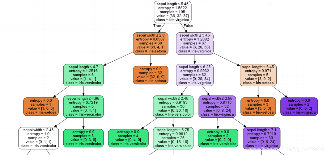
model = DecisionTreeClassifier(criterion='entropy')  # 用ID3
model.fit(x_train, y_train)
y_pred = model.predict(x_test)
print('r^2 score', model.score(x_test, y_test))

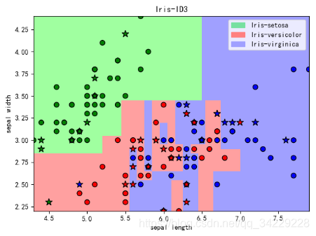
"""可视化"""
light_color = ListedColormap(['#A0FFA0', '#FFA0A0', '#A0A0FF'])
dark_color = ListedColormap(['g', 'r', 'b'])
N = 500
x1_min, x1_max = np.min(x_train[name[0]]), np.max(x_train[name[0]])
x2_min, x2_max = np.min(x_train[name[1]]), np.max(x_train[name[1]])
t1 = np.linspace(x1_min, x1_max, N)
t2 = np.linspace(x2_min, x2_max, N)
x1, x2 = np.meshgrid(t1, t2)
x_new_test = np.stack((x1.flat, x2.flat), axis=1)
y_new_hat = model.predict(x_new_test)

plt.figure()
plt.grid()
plt.pcolormesh(x1, x2, y_new_hat.reshape(N, N), cmap=light_color)
plt.scatter(x_train[name[0]], x_train[name[1]], c=y_train, cmap=dark_color, s=50, edgecolors='k')
plt.scatter(x_test[name[0]], x_test[name[1]], c=y_test, cmap=dark_color, marker='*', s=100, edgecolors='k')
plt.xlim(x1_min, x1_max)
plt.ylim(x2_min, x2_max)
plt.ylabel('{}'.format(name[1]))
plt.xlabel('{}'.format(name[0]))
plt.title('Iris-ID3')
patchs = [mpatches.Patch(color='#77E0A0', label='Iris-setosa'),
          mpatches.Patch(color='#FF8080', label='Iris-versicolor'),
          mpatches.Patch(color='#A0A0FF', label='Iris-virginica')]
plt.legend(handles=patchs, fancybox=True, framealpha=0.8)
plt.show()

""""画图判断树的深度是否过拟合"""
deepth = 15
deep_err = []
for k in range(1, 15):
    model = DecisionTreeClassifier(criterion='entropy', max_depth=k)
    model.fit(x_train, y_train)
    y_pred = model.predict(x_test)
    err = 1 - model.score(x_test, y_test)
    deep_err.append(err)

plt.figure()
plt.scatter(range(1, 15), deep_err, c='blue')
plt.plot(range(1, 15), deep_err, c='red')
plt.xlabel(u'决策树深度', fontsize=12)
plt.ylabel(u'错误率', fontsize=12)
plt.title(u'决策树深度与过拟合', fontsize=12)
plt.show()

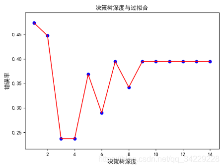
从上图可以看出，当树的深度大于4时，错误率反而上升了，说明发生了过拟合。

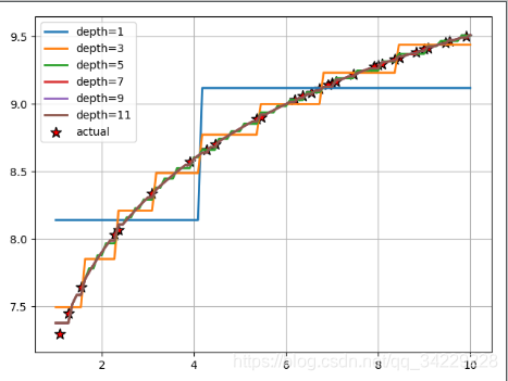
决策树_线性回归

import numpy as np
import matplotlib.pyplot as plt
from sklearn.model_selection import train_test_split
from sklearn.tree import DecisionTreeRegressor

"""先让我造一堆需要回归的数据"""
x = np.linspace(1, 10, 100)+ np.random.random()
y = np.log(x)+ np.random.random()*10
x_train, x_test, y_train, y_test = train_test_split(x, y, train_size=0.7)

"""训练数据"""
depth=12
plt.figure()
for k in range(1,depth,2):
    model=DecisionTreeRegressor(max_depth=k)
    model.fit(x_train.reshape(-1, 1),y_train.reshape(-1, 1))
    x_new_test=np.linspace(1,10,100)
    y_hat=model.predict(x_new_test.reshape(-1, 1))
    plt.plot(np.linspace(1,10,100),y_hat,label='depth={}'.format(k),linewidth=2)
plt.scatter(x_test, y_test, marker='*', c='red', s=100,label='actual',edgecolors='k')
plt.legend(loc='upper left')
plt.grid()
plt.show()

以下图为例，回归是这么做的，假设树的深度为1，指标选为mse，选定阈值为4.1,4,2，对于小于4.1的样本的y求平均得到8.2，大于4.2的样本的y求平均得到9.2，若深度增加则继续往下做，至于阈值的选择（应该是从$x_{min}$-$x_{max}$中随机挑选一个数。）

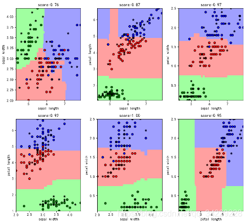
鸢尾花分类_随机森林

import numpy as np
import pandas as pd
import matplotlib.pyplot as plt
from sklearn.model_selection import train_test_split
from sklearn.tree import DecisionTreeClassifier
from sklearn.preprocessing import LabelEncoder
import matplotlib as mpl
from matplotlib.colors import ListedColormap
import matplotlib.patches as mpatches
from sklearn.ensemble import RandomForestClassifier

# 字体
mpl.rcParams['font.sans-serif'] = [u'SimHei']
mpl.rcParams['axes.unicode_minus'] = False

"""读取数据"""
name = ['sepal length', 'sepal width', 'petal length', 'petal width', 'class']
data = pd.read_csv('..\\8.Regression\\iris.data', header=None, names=name)
group = [[0, 1], [0, 2], [0, 3], [1, 2], [1, 3], [2, 3]]
x = data[name[:4]]
y = LabelEncoder().fit_transform(data['class'])

"""init"""
light_color = ListedColormap(['#A0FFA0', '#FFA0A0', '#A0A0FF'])
dark_color = ListedColormap(['g', 'r', 'b'])
N = 500

"""训练数据+可视化"""
plt.figure(figsize=(10, 9), facecolor='#FFFFFF')
plt.grid()
for i, value in enumerate(group):
    print(i, value)

    """将训练集和测试集7|3分"""
    x_train, x_test, y_train, y_test = train_test_split(x.iloc[:, value], y)

    """训练决策树模型"""
    model = RandomForestClassifier(n_estimators=200, criterion='entropy', max_depth=3)  # 用ID3
    model.fit(x_train, y_train)
    y_pred = model.predict(x_test)
    print('r^2 score', model.score(x_test, y_test))

    """可视化"""
    x1_min, x1_max = np.min(x_train.iloc[:, 0]), np.max(x_train.iloc[:, 0])
    x2_min, x2_max = np.min(x_train.iloc[:, 1]), np.max(x_train.iloc[:, 1])
    t1 = np.linspace(x1_min, x1_max, N)
    t2 = np.linspace(x2_min, x2_max, N)
    x1, x2 = np.meshgrid(t1, t2)
    x_new_test = np.stack((x1.flat, x2.flat), axis=1)
    y_new_hat = model.predict(x_new_test)
    
    plt.subplot(2, 3, i + 1)
    plt.pcolormesh(x1, x2, y_new_hat.reshape(N, N), cmap=light_color)
    plt.scatter(x_train.iloc[:, 0], x_train.iloc[:, 1], c=y_train, cmap=dark_color, edgecolors='k')
    plt.scatter(x_test.iloc[:, 0], x_test.iloc[:, 1], c=y_test, cmap=dark_color, marker='*', edgecolors='k')
    plt.xlim(x1_min, x1_max)
    plt.ylim(x2_min, x2_max)
    plt.ylabel('{}'.format(name[value[1]]))
    plt.xlabel('{}'.format(name[value[0]]))
    plt.title('score={:.2f}'.format(model.score(x_test, y_test)))

plt.tight_layout(2.5)
plt.subplots_adjust(top=0.92)
plt.show()