吴恩达cs229|编程作业第一周（Python）

 

练习一：线性回归

 

目录

1.包含的文件

2.单元线性回归

3.多元线性回归

1.包含的文件

文件名	含义
ex1.py	单元线性回归
ex1_multi.py	多元线性回归
ex1data1.txt	单变量线性回归数据集
ex1data2.txt	多变量线性回归数据集
plotData.py	数据可视化
computeCost.py	损失函数
gradientDescent.py	梯度下降
featureNormalize.py	特征归一化
normalEqn.py	正规方程求解线性回归程序

 

红色部分需要自己填写。

2.单元线性回归

项目需要的包

import matplotlib.pyplot as plt
import numpy as np
from matplotlib.colors import LogNorm
from mpl_toolkits.mplot3d import axes3d, Axes3D
from computeCost import *
from gradientDescent import *
from plotData import *
import matplotlib.pyplot as plt

2.1可视化数据集

• 主程序

# ===================== Part 1: Plotting =====================
print('Plotting Data...')


data = np.loadtxt('ex1data1.txt', delimiter=',', usecols=(0, 1))
X = data[:, 0]
y = data[:, 1]
m = y.size


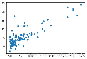
plot_data(X, y)

input('Program paused. Press ENTER to continue')

• 可视化函数plotData.py

import matplotlib.pyplot as plt


def plot_data(x, y):
    # ===================== Your Code Here =====================
    # Instructions : Plot the training data into a figure using the matplotlib.pyplot
    #                using the "plt.scatter" function. Set the axis labels using
    #                "plt.xlabel" and "plt.ylabel". Assume the population and revenue data
    #                have been passed in as the x and y.

    # Hint : You can use the 'marker' parameter in the "plt.scatter" function to change the marker type (e.g. "x", "o").
    #        Furthermore, you can change the color of markers with 'c' parameter.
    plt.scatter(x,y,marker='o',s=50,cmap='Blues',alpha=0.3)  #绘制散点图
    plt.xlabel('population')  #设置x轴标题
    plt.ylabel('profits')   #设置y轴标题
    
    # ===========================================================

    plt.show()

• 运行结果：

2.2梯度下降

• 单变量线性回归的目标是使损失函数最小化：