吴恩达cs229|编程作业第六周（Python）

练习六：支持向量机

目录

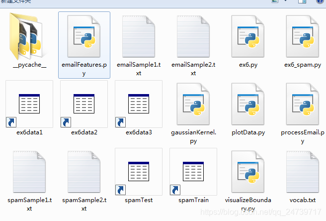
1.包含的文件。

2.支持向量机。

3.垃圾邮件分类。

1.包含的文件。

文件名	含义
ex6.py	支持向量机主程序（第一个实验）
ex6data1.mat	实验1的数据集1
ex6data2.mat	实验1的数据集2
ex6data3.mat	实验1的数据集3
plotData.py	数据集可视化
visualizeBoundary.py	决策边界可视化
gaussianKernel.py	高斯核函数
ex6_spam.py	垃圾邮件分类主程序（第二个实验）
spamTrain.mat	邮件训练集
spamTest.mat	邮件测试集
spamSample1.txt	垃圾邮件事例1
spamSample2.txt	垃圾邮件事例2
vocab.txt	词汇表
emailSample1.txt	邮件事例1
emailSample2.txt	邮件事例2
processEmail.py	邮件预处理
emailFeatures.py	从邮件中提取特征

红色部分需要自己填写。

2.支持向量机

• 加载需要的包和初始化：

import matplotlib.pyplot as plt
import numpy as np
import scipy.io as scio
from sklearn import svm
import plotData as pd
import visualizeBoundary as vb
import gaussianKernel as gk

plt.ion()
np.set_printoptions(formatter={'float': '{: 0.6f}'.format})

2.1绘制数据

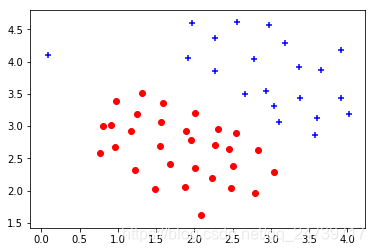
• 编写plotData.py，可视化数据：

import matplotlib.pyplot as plt
import numpy as np

def plot_data(X, y):
    plt.figure()

    # ===================== Your Code Here =====================
    # Instructions : Plot the positive and negative examples on a
    #                2D plot, using the marker="+" for the positive
    #                examples and marker="o" for the negative examples
    #
    count = 0
    for i in y:
        if i == 1:
            plt.scatter(X[count,0],X[count,1],marker='+',color = 'b')
        else:
            plt.scatter(X[count,0],X[count,1],marker='o',color = 'r')
        count = count+1

• 测试代码：

# ===================== Part 1: Loading and Visualizing Data =====================
# We start the exercise by first loading and visualizing the dataset.
# The following code will load the dataset into your environment and
# plot the data

print('Loading and Visualizing data ... ')

# Load from ex6data1:
data = scio.loadmat('ex6data1.mat')
X = data['X']
y = data['y'].flatten()
m = y.size

# Plot training data
pd.plot_data(X, y)

input('Program paused. Press ENTER to continue')

• 测试结果：

2.2训练SVM

• 可视化决策边界visualizeBoundary.py：

def visualize_boundary(clf, X, x_min, x_max, y_min, y_max): #x,y轴的取值范围
    h = .02
    xx, yy = np.meshgrid(np.arange(x_min, x_max, h), np.arange(y_min, y_max, h))#在x，y轴上以0.02为间隔，生成网格点
    Z = clf.predict(np.c_[xx.ravel(), yy.ravel()])#预测每个网格点的类别0/1
    Z = Z.reshape(xx.shape) #转型为网格的形状
    plt.contour(xx, yy,Z, level=[0],colors='r')  #等高线图 将0/1分界线（决策边界）画出来

• 训练线性SVM：