RandLA-Net 亮点1------基于概率的训练样本选取和随机下采样_randla-net中随机点采样的实现-优快云博客

本文链接：https://blog.youkuaiyun.com/qq_24505417/article/details/108977386

RandLA-Net 主要解决两个关键问题: FPS采样耗时和下采样带来的信息丢失.

解决策略: 随机采样(基于概率的训练样本选取和随机下采样) + 局部特征编码(LFA)

RandLA-Net 亮点2——local feature aggregation （LFA）:https://blog.youkuaiyun.com/qq_24505417/article/details/108982154

RandLA-Net Decoder： https://blog.youkuaiyun.com/qq_24505417/article/details/108988259

RandLA-Net训练Semantic3D数据: https://blog.youkuaiyun.com/qq_24505417/article/details/108987171

策略1. 基于概率的训练样本选取和随机下采样

点云数据的预处理工作一直都很大, 很多工作都是对点云进行滑窗+下采样的方式.滑窗方式不可避免的对点云进行了切割,使得原本的物体被切割成几份,破坏了物体的几何形状.而且对于大场景点云数据来说, 滑窗采样工作量非常大.因此RandLA-Net非常巧妙的提出了一个随机采样策略,即能保证快速采样,又能保证均匀采样整个点集. 从而避免一个物体被分成多个部分.

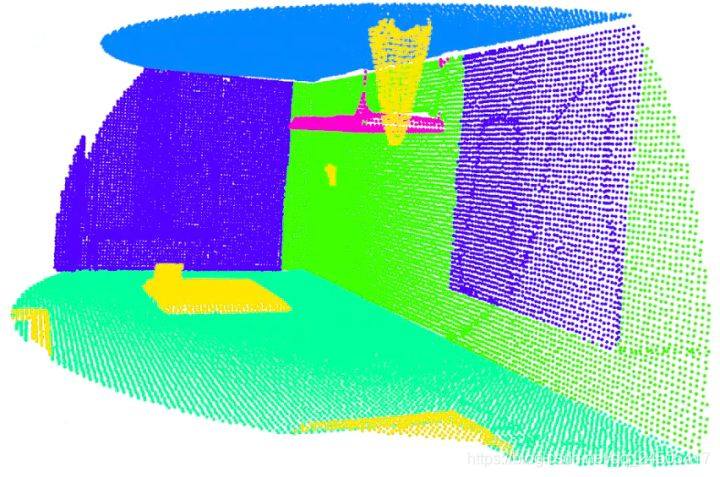
实施细节: 先随机赋予每个点一个概率值,然后从最小概率对应的场景点云中的最小概率点开始,以其为中心,query周边最近的N个点作为一个输入样本点集(包含中心点本身). 对这N个点进行概率更新,使其概率变大,以保证不再采样到此处的点,从而保证在整个点集上均匀采样. 如下图所示

1.预处理( data_prepare_semantic3D.py)
对原始数据(点和标签)进行网格采样, 并生成ply文件和KDTree文件. 同时保存投影信息.

对每个场景分别做数据预处理.

采样:

包括0.01降采样和0.06降采样. 将每个立方体内的点做均值，并统计该立方体内的每个类别的数量，将占比最大的类别作为采样后的类别.

#  Subsample to save space
sub_points, sub_colors, sub_labels = DP.grid_sub_sampling(pc[:,:3].astype(np.float32),\
                               pc[:, 4:7].astype(np.uint8), labels, 0.01)

grid_size = 0.06
sub_xyz, sub_colors, sub_labels = DP.grid_sub_sampling(sub_points, sub_colors, sub_labels, grid_size)

颜色归一化处理:

sub_colors = sub_colors / 255.0

存储为ply文件:原始输入点云为(x,y,z,i,r,g,b)7维信息,网络只使用其中的坐标和颜色信息,再添加一个类别信息一起保存,即(x,y,z,r,g,b,cls),保存格式为ply.

write_ply(sub_ply_file, [sub_xyz, sub_colors, sub_labels], ['x', 'y', 'z', 'red', 'green', 'blue', 'class'])

存储KDTree:同时对0.06降采样后的点云数据构建KDTree,并保存为pkl文件.

search_tree = KDTree(sub_xyz, leaf_size=50)
kd_tree_file = join(sub_pc_folder, file_name + '_KDTree.pkl')

存储投影信息:

 proj_idx = np.squeeze(search_tree.query(sub_points, return_distance=False))
 proj_idx = proj_idx.astype(np.int32)
 proj_save = join(sub_pc_folder, file_name + '_proj.pkl')

2. 样本集生成 (main_Semantic3D.py--->def get_batch_gen())

随机生成概率:

# Random initialize
  for i, tree in enumerate(self.input_trees[split]):
        self.possibility[split] += [np.random.rand(tree.data.shape[0]) * 1e-3]
        self.min_possibility[split] += [float(np.min(self.possibility[split][-1]))]

最小概率场景和该场景下最小概率点:

# Choose the cloud with the lowest probability
 cloud_idx = int(np.argmin(self.min_possibility[split]))

# choose the point with the minimum of possibility in the cloud as query point
 point_ind = np.argmin(self.possibility[split][cloud_idx])

# Get all points within the cloud from tree structure
points = np.array(self.input_trees[split][cloud_idx].data, copy=False)

# Center point of input region
center_point = points[point_ind, :].reshape(1, -1)

搜索N个最近邻:先对中心点添加坐标扰动,然后搜索N个最近点(包含中心店自身)并打乱,然后从整个场景中取出这片点云. semantic3d数据的 N= 65536.打乱的目的是在点云随机采样的时候可以直接取前面的.

# Add noise to the center point
noise = np.random.normal(scale=cfg.noise_init / 10, size=center_point.shape)
pick_point = center_point + noise.astype(center_point.dtype)
query_idx = self.input_trees[split][cloud_idx].query(pick_point, k=cfg.num_points)[1][0]

# Shuffle index
query_idx = DP.shuffle_idx(query_idx)

# Get corresponding points and colors based on the index
queried_pc_xyz = points[query_idx]
ueried_pc_xyz[:, 0:2] = queried_pc_xyz[:, 0:2] - pick_point[:, 0:2]
queried_pc_colors = self.input_colors[split][cloud_idx][query_idx]
if split == 'test':
   queried_pc_labels = np.zeros(queried_pc_xyz.shape[0])
   queried_pt_weight = 1
else:
   queried_pc_labels = self.input_labels[split][cloud_idx][query_idx]
   queried_pc_labels = np.array([self.label_to_idx[l] for l in queried_pc_labels])
   queried_pt_weight = np.array([self.class_weight[split][0][n] for n in queried_pc_labels])

更新概率: 被取出过的点会根据距离信息得到一个概率,以免再次取到此区域

# Update the possibility of the selected points
dists = np.sum(np.square((points[query_idx] - pick_point).astype(np.float32)), axis=1)
delta = np.square(1 - dists / np.max(dists)) * queried_pt_weight
self.possibility[split][cloud_idx][query_idx] += delta
self.min_possibility[split][cloud_idx] = float(np.min(self.possibility[split][cloud_idx]))

上述过程即为收集一个训练样本的过程,.再次搜寻最小概率场景和最小点,重复num_per_epoch = train_steps * batch_size次,即可得到一个epoch所需要的样本数据.

3. 为每层网络事先得到下采样点集以及插值点索引

随着网络加深,点云数量减少, 感受野会逐渐变大, 从而得到全局信息. 因此训练之前记录每个layer的输入点云坐标和他们的N个邻居点,可以提高训练速度.

为输入点集batch_xyz中的每一个点搜索最近点,存储索引为neigh_idx,
因为batch_xyz是打乱过的,所以直接取前1/4 或者1/2即可,采样后保留点集坐标为sub_points, 五个layers的采样率为(4,4,4,4,2). 并没有采用FPS方式采样.
up_i 为每个采样后的点寻找在采样前点集batch_xyz中的最近点. 插值是直接作为新点特征使用.与pointnet++的最近邻插值不同.

for i in range(cfg.num_layers):
    neigh_idx = tf.py_func(DP.knn_search, [batch_xyz, batch_xyz, cfg.k_n], tf.int32)
    sub_points = batch_xyz[:, :tf.shape(batch_xyz)[1] // cfg.sub_sampling_ratio[i], :]
    pool_i = neigh_idx[:, :tf.shape(batch_xyz)[1] // cfg.sub_sampling_ratio[i], :]
    up_i = tf.py_func(DP.knn_search, [sub_points, batch_xyz, 1], tf.int32)
    
    input_points.append(batch_xyz)
    input_neighbors.append(neigh_idx)
    input_pools.append(pool_i)
    input_up_samples.append(up_i)
    batch_xyz = sub_points

网络大致结构如下:

'''
# batch_xyz (B,N,3) sub_sampling_ratio = [4, 4, 4, 4, 2] d_out = [16, 64, 128, 256, 512] 

先用全连接提升到8维,然后进行5次下采样和5次上采样.


点数变化:                                               
                                                    ----->拼接第1层输出特征------>(65536,32+32)->(40960,32) 注意第1层特征用了两次
编码   输入                        输出                (16384,32) ->插值-> (65536,32)
第1层:(65536,8) -> (65536,32) -> (16384,32)          ----->拼接第1层输出特征------>(16384,128+32)->(16384,32)
                                                    (4096,128) ->插值-> (16384,128)
第2层:(16384,32) -> (16384,128) -> (4096,128)          ----->拼接第2层输出特征------>(4096,256+128)->(4096,128)
                                                    (1024,256) ->插值-> (4096,256) 
第3层:(4096,128) -> (4096,256) -> (1024,256)            ----->拼接第3层输出特征------>(1024,512+256)->(1024,256)
                                                    (256,512) ->插值-> (1024,512) 
第4层:(1024,256) -> (1024,512) -> (256,512)             ----->拼接第4层输出特征------>(256,1024+512)->(256,512)
                                                    (128,1024) ->插值-> (256,1024) 
第5层:(256,512) -> (256,1024) -> (128,1024)   ->MLP-> (128,1024)         
                                                    解码
解码后:
(65536,32) -> (65536,64) -> (65536,num_classes)
'''